R: Brunner-Munzel検定をためす：Taglibro de H：SSブログ

	ブログをはじめるログイン

2018日本生態学会大会5日目｜萩原淳一郎『基礎からわかる時系列分析』ブログトップ

R: Brunner-Munzel検定をためす　[統計] [編集]

先日の生態学会の粕谷さんの講演でもふれられていましたが、不等分散のときにMann-WhitneyのU検定（Wilcoxonの順位和検定）をしている例はわりとよく目にします（不等分散のときにつかえない理由はKuboLog 2005-01-29など）。

そういうわけで、Brunner-Munzel検定をためしてみました。やっていることはhoxo_mさんの「マイナーだけど最強の統計的検定 Brunner-Munzel 検定」の後追いです。purrrの練習かもしれません。

まずは正規分布の場合です。平均が同じで分散の異なる分布で、サンプルサイズをかえてためしてみました。以下はRによるコードです。

library(ggplot2)
library(purrr)
library(dplyr)
library(lawstat)

# 正規分布
test_norm <- function(R = 2000, N = c(30, 30),
                      mu = c(0, 0), sigma = c(1, 1)) {
  y <- purrr::map(seq_len(R), function(i) {
    x1 <- rnorm(N[1], mean = mu[1], sd = sigma[1])
    x2 <- rnorm(N[2], mean = mu[2], sd = sigma[2])
    wl <- wilcox.test(x1, x2)$p.value
    bm <- brunner.munzel.test(x1, x2)$p.value
    c(wl, bm)
  })
  df <- data.frame(p_value = purrr::simplify(y),
                   method = rep(c("Wilcoxon", "BM"), R))
  plot <- ggplot(df, aes(p_value, fill = method)) +
    geom_histogram(binwidth = 0.05, boundary = -0.5,
                   position = "dodge")
  print(plot)
  summary <- df %>%
    dplyr::mutate(lt5 = if_else(p_value < 0.05, 1 / (n() / 2), 0)) %>%
    dplyr::group_by(method) %>%
    dplyr::summarize_at("lt5", sum)
  print(summary)
}

set.seed(20180316)
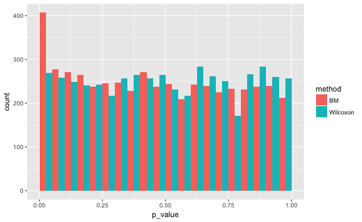
test_norm(R = 5000, N = c(15, 45), mu = c(0, 0), sigma = c(1, 4))
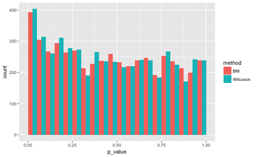
test_norm(R = 5000, N = c(30, 30), mu = c(0, 0), sigma = c(1, 4))
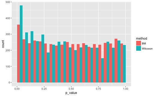
test_norm(R = 5000, N = c(45, 15), mu = c(0, 0), sigma = c(1, 4))

一方の分散を1、他方を4として、p値の分布をシミュレーションで計算しました。

結果です。N = c(15, 45)のとき

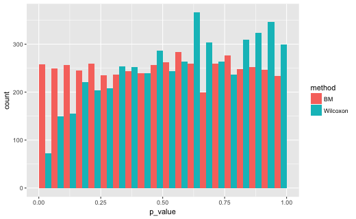
p<0.05となった割合です。

# A tibble: 2 x 2
    method    lt5
      
1       BM 0.0516
2 Wilcoxon 0.0144

N = c(30, 30)のとき

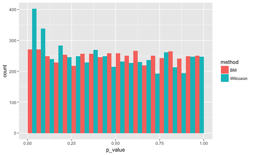
# A tibble: 2 x 2
    method    lt5
      
1       BM 0.0542
2 Wilcoxon 0.0804

N = c(45,15)のとき

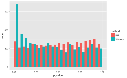
# A tibble: 2 x 2
    method    lt5
      
1       BM 0.0552
2 Wilcoxon 0.1352

Brunner-Munzelの方は、p<0.05となる割合がだいたい0.05となっています。一方、U検定（Wilcoxonの順位和検定）の方は、分散とサンプルサイズの組み合わせより変化しました。

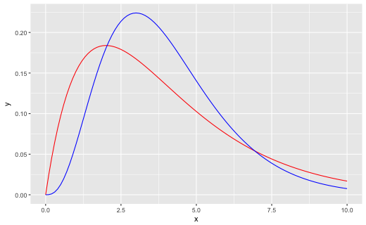
つづいて、ガンマ分布でためしました。下のような分布で比較しました。

# ガンマ分布
shape <- c(2, 4)
scale <- c(2, 1)
ggplot(data.frame(x = seq(0, 10, 0.01)), aes(x)) +
  stat_function(col = "red", fun = dgamma,
                args = list(shape = shape[1], scale = scale[1])) +
  stat_function(col = "blue", fun = dgamma,
                args = list(shape = shape[2], scale = scale[2]))

テストコードです。

test_gamma <- function(R = 2000, N = c(30, 30),
                       shape = c(2, 4), scale = c(2, 1)) {
  y <- purrr::map(seq_len(R), function(i) {
    x1 <- rgamma(N[1], shape = shape[1], scale = scale[1])
    x2 <- rgamma(N[2], shape = shape[2], scale = scale[2])
    wl <- wilcox.test(x1, x2)$p.value
    bm <- brunner.munzel.test(x1, x2)$p.value
    c(wl, bm)
  })
  df <- data.frame(p_value = purrr::simplify(y),
                   method = rep(c("Wilcoxon", "BM"), R))
  plot <- ggplot(df, aes(p_value, fill = method)) +
    geom_histogram(binwidth = 0.05, boundary = -0.5,
                   position = "dodge")
  print(plot)
  summary <- df %>%
    dplyr::mutate(lt5 = if_else(p_value < 0.05, 1 / (n() / 2), 0)) %>%
    dplyr::group_by(method) %>%
    dplyr::summarize_at("lt5", sum)
  print(summary)
}

set.seed(20180316)
test_gamma(R = 5000, N = c(45, 15), shape = shape, scale = scale)
test_gamma(R = 5000, N = c(30, 30), shape = shape, scale = scale)
test_gamma(R = 5000, N = c(15, 45), shape = shape, scale = scale)

結果です。N = c(45, 15)のとき

# A tibble: 2 x 2
    method    lt5
      
1       BM 0.0814
2 Wilcoxon 0.0538

N = c(30, 30)のとき

# A tibble: 2 x 2
    method    lt5
      
1       BM 0.0786
2 Wilcoxon 0.0806

N = c(15,45)のとき

# A tibble: 2 x 2
    method    lt5
      
1       BM 0.0720
2 Wilcoxon 0.0956

この場合、比較している分布の中央値は多少ちがっていますし、群間の平均順位も微妙にちがっているかもしれません。Brunner-Munzel検定でp<0.05となった割合が0.07〜0.08となったのはそのためかとおもわれます。一方、U検定（Wilcoxonの順位和検定）では、やはりサンプルサイズと分散の組み合わせにより、p<0.05となった割合が変化しています。

参考にしたところ