R: 『ポアソン分布・ポアソン回帰・ポアソン過程』のグラフをRで再現してみる(1)

ふと、島谷健一郎『ポアソン分布・ポアソン回帰・ポアソン過程』のグラフをRで再現してみようとおもいたったので、第1章のはじめの方をやってみたメモです。

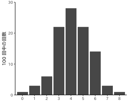
まずは2項分布から はいっています。長さ2の中にイベントをランダムに配置し、前半（1未満）を個数をかぞえるという設定です。

library(ggplot2)
library(dplyr)
set.seed(1)

# 図1.1
sim1 <- function(R = 100, N = 8, L = 2, M = 1) {
  x <- replicate(R, sum(runif(N, 0, L) < M))
  max.count <- max(summary(factor(x)))
  ord <- 10^floor(log10(max.count))
  up <- (max.count %/% ord + 1) * ord
  data.frame(x = factor(x)) %>%
    ggplot(mapping = aes(x = x)) +
    geom_bar() +
    labs(x = "", y = paste(R, "回中の回数")) +
    scale_x_discrete(breaks = 0:N, labels = 0:N) +
    scale_y_continuous(limits = c(0, up), expand = c(0, 0)) +
    theme_classic(base_family = "IPAexGothic")
}

# 1.1(a)
sim1(100, 8, 2, 1)
# 1.1(b)
sim1(100, 8, 2, 1)
# 1.1(c)
sim1(100, 8, 2, 1)

図1.1(a)

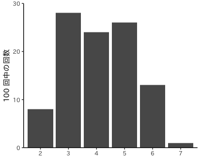
図1.1(b)

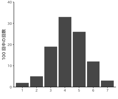
図1.1(c)

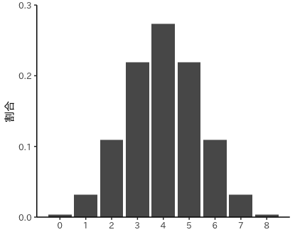
同様の操作を1000回、10000万回繰り返します。図1.2(e)は理論値です。

# 図1.2

# 1.2(a)
sim1(1000, 8, 2, 1)
# 1.2(b)
sim1(1000, 8, 2, 1)

# 1.2(c)
sim1(10000, 8, 2, 1)
# 1.2(d)
sim1(10000, 8, 2, 1)

dsim1 <- function(N, p = 0.5) {
  df <- data.frame(x = 0:N,
                  q = sapply(0:N, function(x) dbinom(x, N, p)))
  up <- floor(max(df$q) / 0.1 + 1) * 0.1
  ggplot(data = df, mapping = aes(x = x, y = q)) +
    geom_bar(stat = "identity") +
    labs(x = "", y = "割合") +
    scale_x_continuous(breaks = 0:N, labels = 0:N) +
    scale_y_continuous(limits = c(0, up), expand = c(0, 0)) +
    theme_classic(base_family = "IPAexGothic")
}

# 1.2(e)
dsim1(8)

図1.2(a)

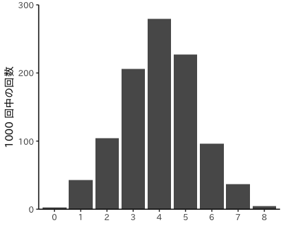
図1.2(b)

図1.2(c)

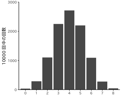
図1.2(d)

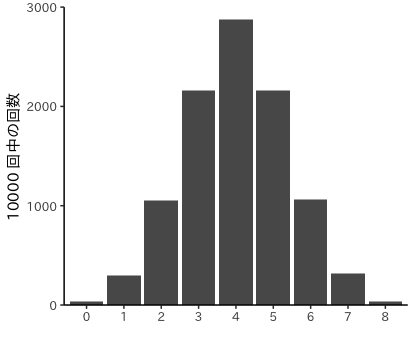
図1.2(e)

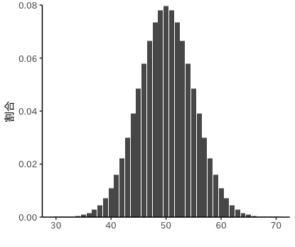
1.3(a)は、面積100の正方形に100個の点をランダムに配置し、左半分に はいった点の数の割合です。1.3(b)は2項分布からの期待値です。

# 図1.3
sim2 <- function(R, N = 100, L = 10, M = 5) {
  x <- replicate(R, sum(runif(N, 0, L) < M))
  h <- hist(x, breaks = min(x):(max(x) + 1),
            include.lowest = FALSE, right = FALSE, plot = FALSE)
  df <- data.frame(range.x = h$breaks[-length(h$breaks)],
                   dens = h$density)
  ord <- 10^floor(log10(max(df$dens)))
  up <- (max(df$dens) %/% ord + 1) * ord
  df %>%
    ggplot(mapping = aes(x = range.x, y = dens)) +
    geom_bar(stat = "identity") +
    labs(x = "", y = "割合") +
    scale_y_continuous(limits = c(0, up), expand = c(0, 0)) +
    theme_classic(base_family = "IPAexGothic")
}

# 1.3(a)
sim2(100, 100)

dsim2 <- function(N, p = 0.5, title = "") {
  df <- data.frame(x = 0:N,
                   q = sapply(0:N, function(x) dbinom(x, N, p))) %>%
    filter(q > 0.00001)
  ord <- 10^floor(log10(max(df$q)))
  up <- (max(df$q) %/% ord + 1) * ord
  ggplot(data = df, mapping = aes(x = x, y = q)) +
    geom_bar(stat = "identity") +
    labs(x = "", y = "割合", title = title) +
    scale_y_continuous(limits = c(0, up), expand = c(0, 0)) +
    theme_classic(base_family = "IPAexGothic")
}

# 1.3(b)
dsim2(100)

図1.3(a)

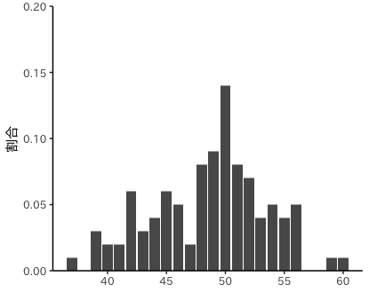
図1.3(b)

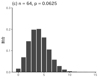
ながさと、はいる割合をかえたときの、2項分布からの期待です。

# 図1.4(a)
dsim2(16, 0.25, title = "(a) n = 16, p = 0.25")
# 図1.4(b)
dsim2(32, 0.125, title = "(b) n = 32, p = 0.125")
# 図1.4(c)
dsim2(64, 0.0625, title = "(c) n = 64, p = 0.0625")

図1.4(a)

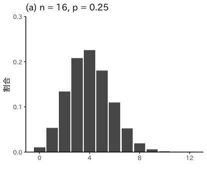
図1.4(b)

図1.4(c)

タグ：R