『ポアソン分布・ポアソン回帰・ポアソン過程』をRで再現してみる(7) [統計]
点配置の比較をしてみます。Stanをつかいます。
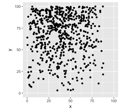
まずは比較対象の点配置を生成します。図5.2(b)の非定常ポアソン過程と同様のものとします。
### 5.6
## Stanによるパラメーター推定
library(ggplot2)
library(dplyr)

## データを生成
set.seed(1)
r <- function(x, y) {
  (-0.00002 * (x - 40)^2 + 0.05) * 0.04 * y
}

x.min <- 0
x.max <- 100
y.min <- 0
y.max <- 100
opt <- optim(par = c(1, 1),
             fn = function(par) -r(par[1], par[2]),
             method = "L-BFGS-B",
             lower = c(x.min, y.min),
             upper = c(x.max, y.max))
r.S <- -opt$value
N <- rpois(1, r.S * (x.max - x.min) * (y.max - y.min))

## 非定常ポアソン過程で点を生成
df <- data.frame(x = runif(N, x.min, x.max),
                 y = runif(N, y.min, y.max),
                 r = runif(N, 0, 1)) %>%
  filter(r(x, y) / r.S > r) %>%
  select(x, y)

ggplot(data = df, mapping = aes(x = x, y = y)) +
  geom_point() +
  xlim(x.min, x.max) +
  ylim(y.min, y.max) +
  coord_equal() +
  theme(aspect.ratio = 1)
こまかく分割した領域を生成します。
n <- c(100, 100)
lx <- (x.max - x.min) / n[1]
ly <- (y.max - y.min) / n[2]

w <- expand.grid(x = seq(x.min + lx / 2, x.max - lx / 2, lx),
                 y = seq(y.min + ly / 2, y.max - ly / 2, ly))
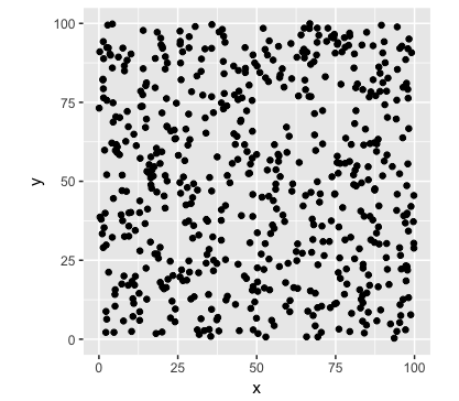
比較する点配置を生成します。こちらは定常ポアソン過程とします。
## 定常ポアソン過程で点を生成
set.seed(2)
np <- rpois(1, nrow(df))
px <- runif(np, x.min, x.max)
py <- runif(np, y.min, y.max)
df2 <- data.frame(x = px, y = py)

ggplot(data = df2, mapping = aes(x = x, y = y)) +
  geom_point() +
  xlim(x.min, x.max) +
  ylim(y.min, y.max) +
  coord_equal() +
  theme(aspect.ratio = 1)
配置を比較します。推定するのはa0とa1というパラメーターで、a1>0ならば配置はかさなり、a1<0ならばたがいに背反の傾向にあるということになります。Stanコードは本の数式をだいたいそのままうつしてあります(というつもりです)。
Stanコード(ipp.stan)
functions {
  real f(vector p, real sigma) {
    real ret = exp(-(p[1]^2 + p[2]^2) / (2 * pi() * sigma^2))
      / (2 * pi() * sigma^2);
    return ret;
  }

  vector k(matrix x, matrix p, matrix u, real sigma) {
    vector[dims(x)[1]] s;
    vector[dims(x)[1]] fout;
    for (j in 1:dims(x)[1]) {
      s[j] = 0;
      for (i in 1:dims(p)[1])
        s[j] = s[j] + f(x[j]' - p[i]', sigma);
      fout[j] = 0;
      for (i in 1:dims(u)[1])
        fout[j] = fout[j] + f(u[i]' - x[j]', sigma);
    }
    return s ./ fout;
  }
}

data {
  int<lower = 0> NX;
  int<lower = 0> NP;
  int<lower = 0> NU;
  matrix[NX, 2] X;
  matrix[NP, 2] P;
  matrix[NU, 2] U;
  real<lower = 0> E;
  real<lower = 0> sigma;
}

transformed data {
  vector[NU] kU = k(U, P, U, sigma);
  vector[NX] kX = k(X, P, U, sigma);
}

parameters {
  real a0;
  real a1;
}

model {
  target += -sum(exp(a0 + a1 * kU) * E) + sum(a0 + a1 * kX);
}
Rコードです。
## RStan
library(rstan)
rstan_options(auto_write = TRUE)
options(mc.cores = parallel::detectCores())

fit2 <- stan("ipp.stan",
             data = list(NX = nrow(df2),
                         NP = nrow(df),
                         NU = nrow(w),
                         X = as.matrix(df2),
                         P = as.matrix(df),
                         U = as.matrix(w),
                         E = lx * ly,
                         sigma = 2),
             iter = 2000, warmup = 1000, thin = 1)
print(fit2)
結果です。a1はだいたい0に近い値となりました。
Inference for Stan model: ipp.
4 chains, each with iter=2000; warmup=1000; thin=1;
post-warmup draws per chain=1000, total post-warmup draws=4000.

         mean se_mean   sd     2.5%      25%      50%      75%    97.5% n_eff
a0      -2.85    0.00 0.06    -2.98    -2.89    -2.85    -2.81    -2.74  1391
a1       0.10    0.02 0.71    -1.31    -0.38     0.10     0.58     1.48  1414
lp__ -2235.28    0.03 1.02 -2238.08 -2235.69 -2234.95 -2234.56 -2234.30  1422
     Rhat
a0      1
a1      1
lp__    1
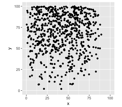
つぎに、同じ非定常ポアソン過程で生成させた配置と比較してみます。
## 同じ非定常ポアソン過程で点を生成
set.seed(3)
N <- rpois(1, r.S * (x.max - x.min) * (y.max - y.min))
df3 <- data.frame(x = runif(N, x.min, x.max),
                 y = runif(N, y.min, y.max),
                 r = runif(N, 0, 1)) %>%
  filter(r(x, y) / r.S > r) %>%
  select(x, y)

data.frame(df3) %>%
  ggplot(mapping = aes(x = x, y = y)) +
  geom_point() +
  xlim(x.min, x.max) +
  ylim(y.min, y.max) +
  coord_equal() +
  theme(aspect.ratio = 1)
fit3 <- stan("ipp.stan",
             data = list(NX = nrow(df3),
                         NP = nrow(df3),
                         NU = nrow(w),
                         X = as.matrix(df3),
                         P = as.matrix(df3),
                         U = as.matrix(w),
                         E = lx * ly,
                         sigma = 2),
             iter = 2000, warmup = 1000, thin = 1)
print(fit3)
結果です。a1は14くらいと推定されました。
Inference for Stan model: ipp.
4 chains, each with iter=2000; warmup=1000; thin=1;
post-warmup draws per chain=1000, total post-warmup draws=4000.

         mean se_mean   sd     2.5%      25%      50%      75%    97.5% n_eff
a0      -4.04    0.00 0.08    -4.19    -4.09    -4.04    -3.98    -3.88  1130
a1      14.14    0.02 0.56    13.02    13.75    14.13    14.52    15.22  1141
lp__ -2200.68    0.02 0.93 -2203.29 -2201.07 -2200.39 -2200.02 -2199.77  1521
     Rhat
a0      1
a1      1
lp__    1


コメント 0