[Stan] 分散を階層化したモデル

分散を階層化したモデルのメモ。

データの生成。

set.seed(12)
n1 <- 80
n2 <- 5

mu <- 0
sigma.bar <- 1.2
sigma.v <- 1.2

sigma <- rgamma(n2, shape = sigma.bar^2 / sigma.v,
                rate = sigma.bar / sigma.v)
y <- sapply(1:n1, function(i) rnorm(n2, mu, sigma))

sigmaの値は以下のとおり。

> print(sigma)
[1] 0.009288378 0.280177830 1.348263631 0.469205587 0.613759563

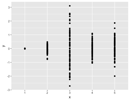
生成されたデータ。

Stanのコード

data {
  int<lower=0> N;
  int<lower=0> M;
  matrix[N, M] Y;
}

parameters {
  vector[M] mu;
  vector<lower=0>[M] sigma;
  real<lower=0> sigma_bar;
  real<lower=0> sigma_v;
}

model {
  real shape = square(sigma_bar) / sigma_v;
  real rate = sigma_bar / sigma_v;

  sigma_bar ~ cauchy(0, 5);
  sigma_v ~ cauchy(0, 5);

  for (j in 1:M)
    sigma[j] ~ gamma(shape, rate);
  for (i in 1:N)
    Y[i] ~ normal(mu, sigma);
}

RStanであてはめ。

fit <- stan("heteroscedasticity.stan",
            data = list(N = n1,
                        M = n2,
                        Y = t(y)),
            control = list(adapt_delta = 0.9))

結果。

> print(fit)
Inference for Stan model: heteroscedasticity.
4 chains, each with iter=2000; warmup=1000; thin=1; 
post-warmup draws per chain=1000, total post-warmup draws=4000.

            mean se_mean    sd   2.5%    25%    50%    75%  97.5% n_eff Rhat
mu[1]       0.00    0.00  0.00   0.00   0.00   0.00   0.00   0.00  4000    1
mu[2]      -0.06    0.00  0.03  -0.12  -0.08  -0.06  -0.04   0.00  4000    1
mu[3]      -0.09    0.00  0.15  -0.38  -0.18  -0.09   0.01   0.19  4000    1
mu[4]       0.00    0.00  0.05  -0.11  -0.04  -0.01   0.03   0.10  4000    1
mu[5]       0.05    0.00  0.07  -0.09   0.00   0.05   0.10   0.20  4000    1
sigma[1]    0.01    0.00  0.00   0.01   0.01   0.01   0.01   0.01  4000    1
sigma[2]    0.26    0.00  0.02   0.22   0.25   0.26   0.27   0.31  4000    1
sigma[3]    1.32    0.00  0.11   1.14   1.25   1.32   1.39   1.56  4000    1
sigma[4]    0.49    0.00  0.04   0.42   0.46   0.48   0.51   0.57  4000    1
sigma[5]    0.67    0.00  0.05   0.57   0.63   0.67   0.70   0.79  4000    1
sigma_bar   1.41    0.02  0.84   0.44   0.87   1.24   1.74   3.32  2133    1
sigma_v     6.69    0.46 20.17   0.31   1.46   3.12   6.79  34.22  1951    1
lp__      349.21    0.06  2.46 343.41 347.74 349.47 350.99 353.05  1500    1

Samples were drawn using NUTS(diag_e) at Fri Feb 17 20:57:24 2017.
For each parameter, n_eff is a crude measure of effective sample size,
and Rhat is the potential scale reduction factor on split chains (at 
convergence, Rhat=1).

sigma_vの事後分布がいまひとつだが、それ以外はだいたいうまく推定できている。

タグ：STAn