R: KFASによる状態空間モデル (4)

きょうは季節調整モデル。

library(ggplot2)
library(KFAS)

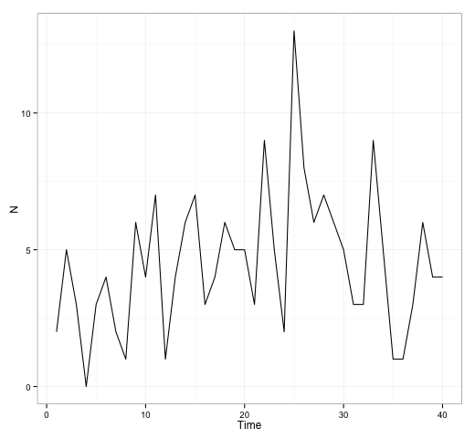
データ生成。

set.seed(17)
N.t <- 40                    # 測定回数
season <- c(0, 0.3, 0, -0.3) # 季節調整成分
alpha <- rep(NA, N.t)         # 個体数の対数
alpha[1] <- 1 + season[1 %% 4 + 1]
for (t in 2:N.t) {
  alpha[t] <- rnorm(1, alpha[t - 1], 0.05) + season[t %% 4 + 1]
}
N <- rpois(N.t, exp(alpha))

グラフを表示。

df <- data.frame(Time = 1:N.t, N = N)
p5 <- ggplot(df, aes(x = Time, y = N)) +
      geom_line() +
      theme_bw()
print(p5)

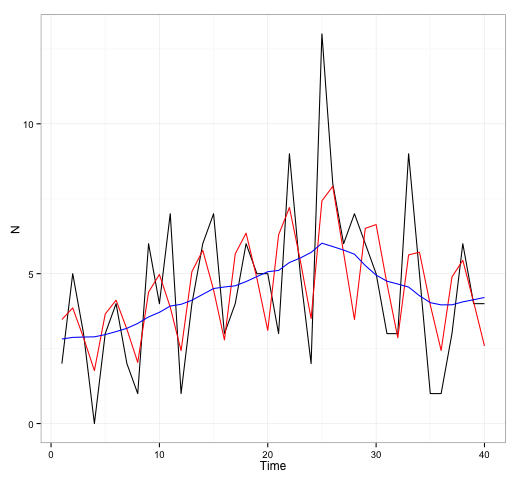
ローカルレベルモデル+季節調整モデル。

## KFAS
## Local Level Model + Seasonal 
model3 <- SSModel(N ~ SSMtrend(degree = 1, Q = list(NA)) +
                      SSMseasonal(period = 4, Q = NA, sea.type = "dummy"),
                  data = df,
                  distribution = "poisson")
fit3 <- fitSSM(model = model3, inits = c(1, 1), method = "BFGS")
out3 <- KFS(fit3$model, smoothing = c("state", "mean"))

季節調整成分ふくめて平滑化したものと、トレンド成分の信号のみをとりだして測定値のスケールになおしたものを重ねてプロット。

## Signal
df$Smoothed <- fitted(out3)
df$Trend <- exp(c(signal(out3, states = "trend")$signal))
p6 <- ggplot(df) +
      geom_line(aes(x = Time, y = N), color = "black") +
      geom_line(aes(x = Time, y = Smoothed), color = "red") + 
      geom_line(aes(x = Time, y = Trend), color = "blue") +
      theme_bw()
print(p6)

タグ：KFAS R