R: nlme

nlmeはあまりつかったことがなかった。のでちょっとテストしてみた。

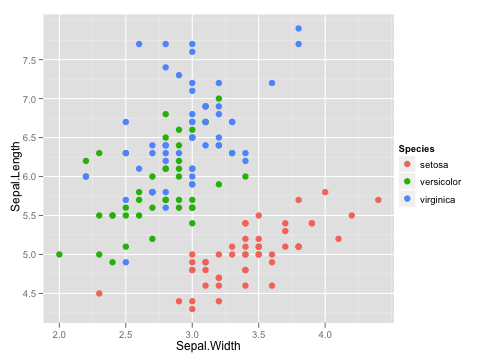
ネタとして適当かどうかわからないが、data(iris)を使用。

library(ggplot2)
data(iris)
p <- ggplot(iris, aes(x = Sepal.Width, y = Sepal.Length))
p1 <- p + geom_point(aes(color = Species), size = 3)
print(p1)

べき乗式をあてはめてみる。

library(nlme)

sepal.nlme1 <- nlme(Sepal.Length ~ a * Sepal.Width^b,
                    data = iris,
                    fixed = a + b ~ 1,
                    random = a + b ~ 1|Species,
                    start = c(1, 1), method = "ML")
summary(sepal.nlme1)

結果

Nonlinear mixed-effects model fit by maximum likelihood
  Model: Sepal.Length ~ a * Sepal.Width^b 
 Data: iris 
       AIC      BIC    logLik
  204.2433 222.3071 -96.12165

Random effects:
 Formula: list(a ~ 1, b ~ 1)
 Level: Species
 Structure: General positive-definite, Log-Cholesky parametrization
         StdDev     Corr  
a        0.62713825 a     
b        0.03333759 -0.999
Residual 0.43627681       

Fixed effects: a + b ~ 1 
     Value Std.Error  DF  t-value p-value
a 3.635606 0.4274668 146 8.505004       0
b 0.433948 0.0583800 146 7.433155       0
 Correlation: 
  a     
b -0.773

Standardized Within-Group Residuals:
        Min          Q1         Med          Q3         Max 
-2.86192796 -0.58150305 -0.07887569  0.43579445  3.33264845 

Number of Observations: 150
Number of Groups: 3 

Random effectsにおけるaとｂとの相関が-0.999なので、たぶんどちらか一方だけでよい。

sepal.nlme2 <- nlme(Sepal.Length ~ a * Sepal.Width^b,
                    data = iris,
                    fixed = a + b ~ 1,
                    random = a ~ 1|Species,
                    start = c(1, 1), method = "ML")
summary(sepal.nlme2)

結果

Nonlinear mixed-effects model fit by maximum likelihood
  Model: Sepal.Length ~ a * Sepal.Width^b 
 Data: iris 
       AIC      BIC    logLik
  200.4443 212.4869 -96.22217

Random effects:
 Formula: a ~ 1 | Species
                a  Residual
StdDev: 0.5005274 0.4365705

Fixed effects: a + b ~ 1 
     Value Std.Error  DF  t-value p-value
a 3.662996 0.3687761 146 9.932843       0
b 0.423954 0.0555806 146 7.627739       0
 Correlation: 
  a     
b -0.612

Standardized Within-Group Residuals:
        Min          Q1         Med          Q3         Max 
-2.80406587 -0.60478687 -0.05863561  0.43341116  3.37435711 

Number of Observations: 150
Number of Groups: 3 

やはり後者の方がAICが小さい。

ちなみに直線回帰lm()でSpeciesを因子としてモデルに組み込んだ場合は

sepal.lm <- lm(Sepal.Length ~ Sepal.Width + Species,
               data = iris)
summary(sepal.lm)
AIC(sepal.lm)

結果

> summary(sepal.lm)

Call:
lm(formula = Sepal.Length ~ Sepal.Width + Species, data = iris)

Residuals:
     Min       1Q   Median       3Q      Max 
-1.30711 -0.25713 -0.05325  0.19542  1.41253 

Coefficients:
                  Estimate Std. Error t value Pr(>|t|)    
(Intercept)         2.2514     0.3698   6.089 9.57e-09 ***
Sepal.Width         0.8036     0.1063   7.557 4.19e-12 ***
Speciesversicolor   1.4587     0.1121  13.012  < 2e-16 ***
Speciesvirginica    1.9468     0.1000  19.465  < 2e-16 ***
---
Signif. codes:  0 ‘***’ 0.001 ‘**’ 0.01 ‘*’ 0.05 ‘.’ 0.1 ‘ ’ 1 

Residual standard error: 0.438 on 146 degrees of freedom
Multiple R-squared: 0.7259,	Adjusted R-squared: 0.7203 
F-statistic: 128.9 on 3 and 146 DF,  p-value: < 2.2e-16 

> AIC(sepal.lm)
[1] 183.9366

まあ結局、単純なものがよさそう。

タグ：R