MCMC: tauの事前分布 [統計]
Carlin & Louis "Bayesian Methods for Data Analysis (3rd ed.)"の45ページ以降で、分散の逆数tauにあたえる事前分布が論じられている。Gamma(ε, ε)という事前分布を使った場合、選択したεにたいして事後分布が鋭敏になる可能性があるということである。
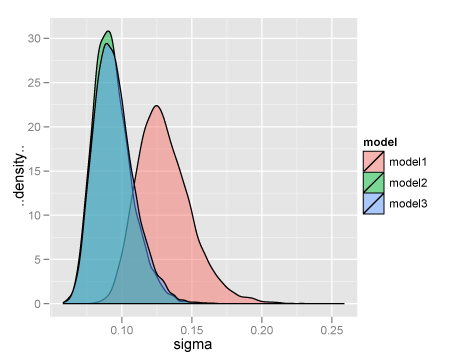
で、例題があったのでためしてみた。model1ではtau ~ dgamma(0.1, 0.1)、model2ではtau ~ dgamma(1.0E-3, 1.0E-3)、model3ではsigma ~ dunif(0.01, 100)としている。
結果
sigmaの事後分布をならべてみる。
ちなみに。
で、例題があったのでためしてみた。model1ではtau ~ dgamma(0.1, 0.1)、model2ではtau ~ dgamma(1.0E-3, 1.0E-3)、model3ではsigma ~ dunif(0.01, 100)としている。
library(R2WinBUGS)

WINE <- "/Applications/Darwine/Wine.bundle/Contents/bin/wine"
WINEPATH <- "/Applications/Darwine/Wine.bundle/Contents/bin/winepath"

model1 <- function() {
  for (i in 1:n) {
    logage[i] <- log(x[i])
    Y[i] ~ dnorm(mu[i], tau)
    mu[i] <- beta0 + beta1 * (logage[i] - mean(logage[]))
  }

  beta0 ~ dflat()
  beta1 ~ dflat()

  tau ~ dgamma(0.1, 0.1)
  sigma <- 1/sqrt(tau)
}
write.model(model1, "model1.bug")

model2 <- function() {
  for (i in 1:n) {
    logage[i] <- log(x[i])
    Y[i] ~ dnorm(mu[i], tau)
    mu[i] <- beta0 + beta1 * (logage[i] - mean(logage[]))
  }

  beta0 ~ dflat()
  beta1 ~ dflat()

  tau ~ dgamma(1.0E-3, 1.0E-3)
  sigma <- 1/sqrt(tau)
}
write.model(model2, "model2.bug")

model3 <- function() {
  for (i in 1:n) {
    logage[i] <- log(x[i])
    Y[i] ~ dnorm(mu[i], tau)
    mu[i] <- beta0 + beta1 * (logage[i] - mean(logage[]))
  }

  beta0 ~ dflat()
  beta1 ~ dflat()

  tau <- 1/(sigma * sigma)
  sigma ~ dunif(0.01, 100)
}
write.model(model3, "model3.bug")

data <- list(
  x = c( 1.0,  1.5,  1.5,  1.5,  2.5,  4.0,  5.0,  5.0,  7.0,
         8.0,  8.5,  9.0,  9.5,  9.5, 10.0, 12.0, 12.0, 13.0,
        13.0, 14.5, 15.5, 15.5, 16.5, 17.0, 22.5, 29.0, 31.5),
  Y = c(1.80, 1.85, 1.87, 1.77, 2.02, 2.27, 2.15, 2.26, 2.47,
        2.19, 2.26, 2.40, 2.39, 2.41, 2.50, 2.32, 2.32, 2.43,
        2.47, 2.56, 2.65, 2.47, 2.64, 2.56, 2.70, 2.72, 2.57),
  n = 27)

init1 <- list(beta0 = 0, beta1 = 1, tau = 1)
init3 <- list(beta0 = 0, beta1 = 1, sigma = 1)

params <- c("beta0", "beta1", "sigma")

post1 <- bugs(data = data, inits = list(init1, init1, init1),
              parameters.to.save = params,
              model.file = "model1.bug",
              n.chains = 3, n.iter = 31000, n.burnin = 1000,
              n.thin = 10, debug = FALSE,
              working.directory = getwd(),
              WINE = WINE, WINEPATH = WINEPATH)

post2 <- bugs(data = data, inits = list(init1, init1, init1),
              parameters.to.save = params,
              model.file = "model2.bug",
              n.chains = 3, n.iter = 31000, n.burnin = 1000,
              n.thin = 10, debug = FALSE,
              working.directory = getwd(),
              WINE = WINE, WINEPATH = WINEPATH)

post3 <- bugs(data = data, inits = list(init3, init3, init3),
              parameters.to.save = params,
              model.file = "model3.bug",
              n.chains = 3, n.iter = 31000, n.burnin = 1000,
              n.thin = 10, debug = FALSE,
              working.directory = getwd(),
              WINE = WINE, WINEPATH = WINEPATH)
結果
> print(post1, digits = 3)
Inference for Bugs model at "model1.bug", fit using WinBUGS,
 3 chains, each with 31000 iterations (first 1000 discarded), n.thin = 10
 n.sims = 9000 iterations saved
            mean    sd    2.5%     25%     50%     75%   97.5%  Rhat n.eff
beta0      2.334 0.025   2.285   2.318   2.334   2.351   2.383 1.001  9000
beta1      0.277 0.028   0.222   0.259   0.277   0.295   0.330 1.002  2400
sigma      0.131 0.019   0.099   0.117   0.128   0.142   0.174 1.001  9000
deviance -46.295 4.800 -53.500 -49.780 -47.025 -43.540 -35.110 1.001  9000

For each parameter, n.eff is a crude measure of effective sample size,
and Rhat is the potential scale reduction factor (at convergence, Rhat=1).

DIC info (using the rule, pD = Dbar-Dhat)
pD = 3.1 and DIC = -43.2
DIC is an estimate of expected predictive error (lower deviance is better).
> print(post2, digits = 3)
Inference for Bugs model at "model2.bug", fit using WinBUGS,
 3 chains, each with 31000 iterations (first 1000 discarded), n.thin = 10
 n.sims = 9000 iterations saved
            mean    sd    2.5%     25%     50%     75%   97.5%  Rhat n.eff
beta0      2.334 0.018   2.299   2.322   2.334   2.346   2.370 1.001  9000
beta1      0.277 0.020   0.239   0.264   0.277   0.290   0.316 1.001  7300
sigma      0.093 0.014   0.071   0.084   0.092   0.101   0.125 1.001  6200
deviance -52.351 2.596 -55.300 -54.230 -53.020 -51.200 -45.620 1.001  9000

For each parameter, n.eff is a crude measure of effective sample size,
and Rhat is the potential scale reduction factor (at convergence, Rhat=1).

DIC info (using the rule, pD = Dbar-Dhat)
pD = 3.1 and DIC = -49.3
DIC is an estimate of expected predictive error (lower deviance is better).
> print(post3, digits = 3)
Inference for Bugs model at "model3.bug", fit using WinBUGS,
 3 chains, each with 31000 iterations (first 1000 discarded), n.thin = 10
 n.sims = 9000 iterations saved
            mean    sd    2.5%     25%     50%     75%   97.5%  Rhat n.eff
beta0      2.334 0.018   2.298   2.322   2.334   2.346   2.369 1.001  6000
beta1      0.277 0.020   0.238   0.264   0.277   0.290   0.317 1.001  9000
sigma      0.095 0.014   0.072   0.084   0.093   0.103   0.128 1.001  9000
deviance -52.245 2.621 -55.270 -54.190 -52.920 -50.970 -45.470 1.001  8400

For each parameter, n.eff is a crude measure of effective sample size,
and Rhat is the potential scale reduction factor (at convergence, Rhat=1).

DIC info (using the rule, pD = Dbar-Dhat)
pD = 2.9 and DIC = -49.4
DIC is an estimate of expected predictive error (lower deviance is better).
sigmaの事後分布をならべてみる。
ちなみに。
> summary(lm(data$Y ~ log(data$x)))

Call:
lm(formula = data$Y ~ log(data$x))

Residuals:
      Min        1Q    Median        3Q       Max
-0.148441 -0.054890  0.004223  0.054358  0.168681

Coefficients:
            Estimate Std. Error t value Pr(>|t|)
(Intercept)  1.76166    0.04250   41.45  < 2e-16 ***
log(data$x)  0.27733    0.01881   14.75  7.7e-14 ***
---
Signif. codes:  0 ‘***’ 0.001 ‘**’ 0.01 ‘*’ 0.05 ‘.’ 0.1 ‘ ’ 1

Residual standard error: 0.08994 on 25 degrees of freedom
Multiple R-squared: 0.8969,	Adjusted R-squared: 0.8928
F-statistic: 217.5 on 1 and 25 DF,  p-value: 7.707e-14
タグ:MCMC


コメント 0