R: drmを使ってみる

順序尺度の目的変数を解析する累積ロジットモデル。drmを使ってみた。混合モデルを解析できる。

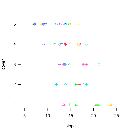
こういうデータを用意。

# inverse logit
invlogit <- function(x) exp(x)/(1+exp(x))

set.seed(123)
plot <- 1:30
n.plot <- length(plot)
time <- 1:3
n.time <- length(time)
data <- expand.grid(plot = plot, time = time)
slope <- rgamma(n.plot, shape = 15^2/5^2, rate = 15/5^2)
data$slope <- rep(slope, n.time)
ranef.plot <- rnorm(n.plot, 0, 1)
ranef.time <- rnorm(n.time, 0, 1)
logit.c1 <- 7.5 - 0.5 * slope +
            ranef.plot[data$plot] + ranef.time[data$time]
data$c1 <- rbinom(n.plot * n.time, 4, invlogit(logit.c1)) + 1

col <- rainbow(n.plot)
plot(c1 ~ slope, data = data, pch = time, col = col[plot],
     las = 1, ylab = "cover", xlim = c(5,30))

drmで解析する。nlmで尤度を最大にしているようだ。(追記) marginal regressionという方法を使用しているようだ。デフォルトの初期値ではうまくいかないことがある。

library(drm)

fit <- drm(c1 ~ slope + cluster(plot) + Time(time),
                data = data,
                start = c(3, 4, 5, 6, -1))
summary(fit)

結果

Call:
drm(formula = c1 ~ slope + cluster(plot) + Time(time), data = data, 
    start = c(3, 4, 5, 6, -1))

Coefficients:
                   Value Std. Error   z value
(Intercept)1 -10.9588098 1.39089022 -7.878990
(Intercept)2  -9.4931094 1.26458408 -7.506903
(Intercept)3  -8.4885088 1.18236774 -7.179246
(Intercept)4  -6.7823769 1.05836034 -6.408382
slope         -0.5746348 0.07889966 -7.283109

Residual deviance: 191.666 	AIC: 201.666 

Convergence code 1 in 27 iterations (See help(nlm) for details)

Correlation of Coefficients:
             (Intercept)1 (Intercept)2 (Intercept)3 (Intercept)4
(Intercept)2        0.965                                       
(Intercept)3        0.952        0.976                          
(Intercept)4        0.931        0.945        0.956             
slope               0.965        0.971        0.970        0.958

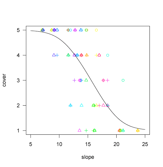
Gelman & Hill (2007) を参考に、期待値の曲線を重ねてみる。

coef <- fit$coefficient
x <- seq(5, 30, 0.1)
expected <- 5 * invlogit(coef[5] * x - coef[4]) +
            4 * (invlogit(coef[5] * x - coef[3]) -
                 invlogit(coef[5] * x - coef[4])) +
            3 * (invlogit(coef[5] * x - coef[2]) -
                 invlogit(coef[5] * x - coef[3])) +
            2 * (invlogit(coef[5] * x - coef[1]) -
                 invlogit(coef[5] * x - coef[2])) +
            1 * (1 - invlogit(coef[5] * x - coef[1]))
lines(x, expected)

タグ：累積ロジットモデル