R: MCMCpackの並列化

ふと、MCMCpackパッケージのMCMCpoisson()関数を並列化してみました。

ポアソン回帰用の模擬データをつくります。

library(MCMCpack)

## Data
set.seed(11)
N <- 201
x <- seq(0, 1, length = N)
y <- rpois(N, exp(3 * x - 1))
d <- data.frame(x = x, y = y)

まずはmclapply()をつかってみます。MCMCpoisson()のseed引数に、要素2つのlistを指定すると、並列化むきというL'Ecuyer random number generatorを使用できます。最初の要素は長さ6のベクトル、2番目の要素はsubstream numberです。詳細はhelp(MCMCpoisson)をご覧ください。

library(parallel)

n.chains <- 3
seeds <- seq.int(from = 11, by = 13, length = 6)
fit <- mclapply(1:n.chains,
                function(ch) {
                  MCMCpoisson(y ~ x, data = d,
                              burnin = 1000, mcmc = 3000, thin = 3,
                              verbose = 0, seed = list(seeds, ch))
                },
                mc.cores = 4)
fit.list <- mcmc.list(fit)
gelman.diag(fit.list)
summary(fit.list)
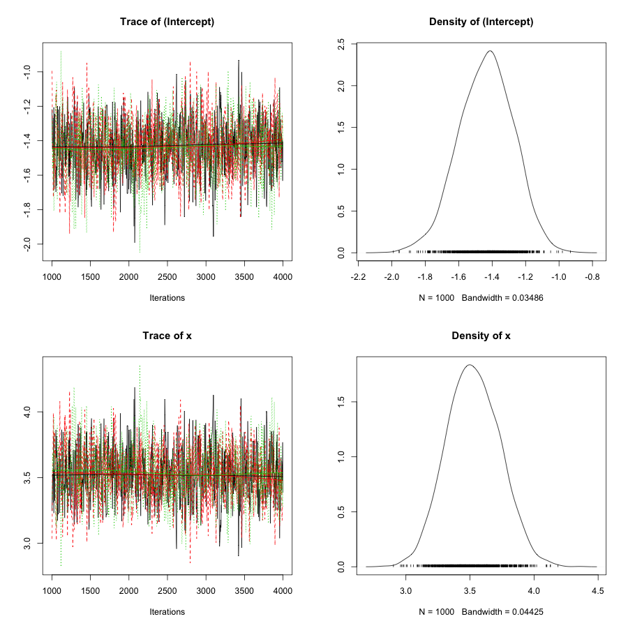
plot(fit.list)

結果です。

> gelman.diag(fit.list)
Potential scale reduction factors:

            Point est. Upper C.I.
(Intercept)          1       1.01
x                    1       1.01

Multivariate psrf

1
> summary(fit.list)

Iterations = 1001:3998
Thinning interval = 3 
Number of chains = 3 
Sample size per chain = 1000 

1. Empirical mean and standard deviation for each variable,
   plus standard error of the mean:

              Mean     SD Naive SE Time-series SE
(Intercept) -1.436 0.1631 0.002978       0.005010
x            3.527 0.2070 0.003780       0.006333

2. Quantiles for each variable:

              2.5%    25%    50%    75%  97.5%
(Intercept) -1.772 -1.548 -1.428 -1.323 -1.126
x            3.138  3.381  3.521  3.670  3.934

つづいて、foreach()で。

##
## foreach
##
library(foreach)
library(doMC)

registerDoMC(4)

fit2 <- foreach(ch = 1:n.chains) %dopar% {
    MCMCpoisson(y ~ x, data = d,
                burnin = 1000, mcmc = 3000, thin = 3,
                verbose = 0, seed = list(seeds, ch))
  }
fit2.list <- mcmc.list(fit2)
gelman.diag(fit2.list)
summary(fit2.list)

結果です。

> gelman.diag(fit2.list)
Potential scale reduction factors:

            Point est. Upper C.I.
(Intercept)          1       1.01
x                    1       1.01

Multivariate psrf

1
> summary(fit2.list)

Iterations = 1001:3998
Thinning interval = 3 
Number of chains = 3 
Sample size per chain = 1000 

1. Empirical mean and standard deviation for each variable,
   plus standard error of the mean:

              Mean     SD Naive SE Time-series SE
(Intercept) -1.436 0.1631 0.002978       0.005010
x            3.527 0.2070 0.003780       0.006333

2. Quantiles for each variable:

              2.5%    25%    50%    75%  97.5%
(Intercept) -1.772 -1.548 -1.428 -1.323 -1.126
x            3.138  3.381  3.521  3.670  3.934

乱数のseedを指定してあるので、結果は一致します。

ただ、これくらいの計算量だと並列化の御利益はありません。

タグ：R MCMC