R: KFASによる実データの解析例：Taglibro de H：SSブログ

	ブログをはじめるログイン

R: KFASによる実データの解析例　[統計] [編集]

KFASをつかって、Bayesian Population Analysis using WinBUGS第3章のハヤブサのデータを状態空間モデルで解析してみる。

library(KFAS)
library(ggplot2)

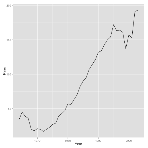
falcons <- read.delim("falcons.txt")
head(falcons)

ggplot(falcons) +
  geom_line(aes(x = Year, y = Pairs))

観測モデルはポアソン分布、プロセスモデル部分は2次のトレンドモデルにあてはめ。

## トレンドモデル
model <- SSModel(Pairs ~ SSMtrend(degree = 2,
                                  Q = list(matrix(NA), matrix(NA))),
                 data = falcons, distribution = "poisson")
## パラメーター推定
fit <- fitSSM(model, inits = c(1, 1), method = "BFGS")

プロセスモデルの分散共分散行列のQを表示。

> fit$model$Q
, , 1

             [,1]        [,2]
[1,] 6.254557e-07 0.000000000
[2,] 0.000000e+00 0.001859009

レベルの分散はちいさい。

つづいて、カルマンフィルターを適用して、状態の値を表示する。

## 状態の表示
out <- KFS(fit$model, smoothing = c("state", "mean"))

値は、観測値の対数スケールになっている。

> coef(out)
Time Series:
Start = 1 
End = 40 
Frequency = 1 
      level        slope
 1 3.722354 -0.101679163
 2 3.620679 -0.115350974
 3 3.505328 -0.128485351
 4 3.376839 -0.130461354
 5 3.246370 -0.108773871
 6 3.137591 -0.074006144
 7 3.063584 -0.035537613
 8 3.028045  0.005883994
 9 3.033929  0.049039924
10 3.082971  0.086906959
11 3.169880  0.116096719
12 3.285981  0.135113842
13 3.421098  0.144450883
14 3.565553  0.141128039
15 3.706683  0.131914101
16 3.838598  0.121050476
17 3.959648  0.109540617
18 4.069186  0.105863778
19 4.175049  0.105355153
20 4.280404  0.104216785
21 4.384623  0.098229391
22 4.482853  0.090724408
23 4.573577  0.084515021
24 4.658092  0.076087655
25 4.734180  0.068352112
26 4.802532  0.061735774
27 4.864267  0.054717204
28 4.918983  0.051802684
29 4.970786  0.047669153
30 5.018457  0.040197003
31 5.058655  0.027196705
32 5.085856  0.002387118
33 5.088241 -0.015117981
34 5.073120 -0.023653628
35 5.049460 -0.015173253
36 5.034278  0.019733345
37 5.054013  0.050228410
38 5.104243  0.076963635
39 5.181215  0.078153433
40 5.259369  0.078153433

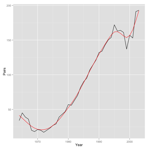
平滑化してみる。

## 平滑化
pred1 <- predict(fit$model, type = "response")

falcons$SmoothedPairs <- pred1

p1 <- ggplot(falcons)
p1 + geom_line(aes(x = Year, y = Pairs)) +
  geom_line(aes(x = Year, y = SmoothedPairs), color = "red")

5年先までの予測。

## 予測
next.year <- max(falcons$Year) + 1
n.prediction <- 5
pred2 <- predict(fit$model, n.ahead = n.prediction, type = "response",
                 interval = "prediction", nsim = 1000)
falcons.pred <- data.frame(Year = next.year:(next.year + n.prediction - 1),
                           Fit = pred2[, "fit"],
                           Lower = pred2[, "lwr"],
                           Upper = pred2[, "upr"])

p1 + geom_line(aes(x = Year, y = Pairs)) +
  geom_line(aes(x = Year, y = SmoothedPairs), color = "red") +
  geom_line(data = falcons.pred,
            aes(x = Year, y = Fit), color = "red") +
  geom_ribbon(data = falcons.pred,
              aes(x = Year, ymin = Lower, ymax = Upper),
              fill = "red", alpha = 0.5)

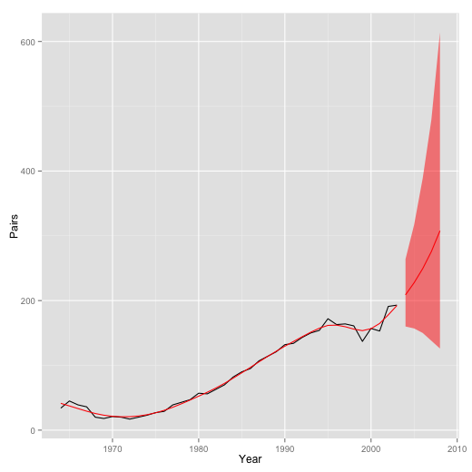
うすい赤色は95%予測区間。予測区間の幅はひろい。

タグ：R KFAS

2015-07-11 13:03 nice!(2) コメント(4) トラックバック(0)
共通テーマ：日記・雑感

nice! 2

状態空間モデル初心者です。参考に勉強させていただいています。ところで、生態学だと、調査回数や調査区の大きさが年度によってちょっと変更になってしまいながらも長期で続けて観測しているデータが多いと思いますが、ＧＬＭのoffset項のような便利な技はＫＦＡＳにはあるのでしょうか？KFAS本体の説明書も読んではいますが、探し切れていません。もし知っていたらブログ上で説明していただけると助かります。
by 初心者 (2016-12-23 13:57)

係数を固定すればよいので、SSMcustom()でなんとかなりそうな気もしますが、Stanとかで実装してしまう方が簡単かもしれません。
by hiroki (2016-12-23 19:47)

初めまして。状態空間モデルの利用を検討しています。上記のsmoothingの引数でstateとmeanの二つを当てていますが、これはどういうことなのでしょうか。KFASのマニュアルでは、デフォルトでこれになっていると書かれているのですが、どうしてそうなのかが分かりませんでした。ご存じなことがありましたら。ご教示いただけますと助かります。
by takaaki (2017-07-12 16:09)

stateの方は状態（この場合は、水準成分と傾き成分）を個別に求め、meanの方はそれらをあわせて、ポアソン分布の場合にはexpを適用した値を計算します。
stateはcoef(out)で、meanはfitted(out)でそれぞれ表示されます。

by hiroki (2017-07-12 19:20)