R: 時系列データ間の関係を状態空間モデルでみる (2)

きのうのつづき。今度は本当に関係のある場合。

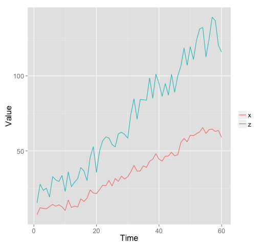
zは、xを2倍してノイズをくわえた値とする。

## zはxから生成
z <- rnorm(N.t, x * 2, 8)
df2 <- data.frame(time = 1:N.t, x = x, z = z)

p2 <- ggplot(df2)
p2 + geom_line(aes(x = rep(time, 2), y = c(x, z),
                   color = rep(c("x", "z"), each = N.t))) +
  xlab("Time") + ylab("Value") +
  guides(color = guide_legend(title = "")) +
  theme_gray(base_size = 16)

p2 + geom_point(aes(x = x, y = z)) +
  theme_gray(base_size = 16)

グラフ

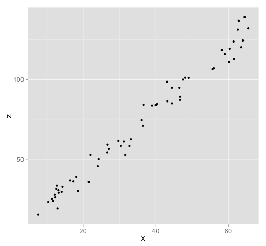
相関をみてみる。

> cor.test(x, z)

	Pearson's product-moment correlation

data:  x and z
t = 30.4594, df = 58, p-value < 2.2e-16
alternative hypothesis: true correlation is not equal to 0
95 percent confidence interval:
 0.9503121 0.9821228
sample estimates:
      cor 
0.9701356 

model3はxとの回帰をふくめないトレンドモデル、model4はxとの回帰をふくめたトレンドモデルとする。

model3 <- SSModel(z ~ SSMtrend(degree = 2,
                               Q = list(matrix(NA), matrix(NA))),
                  data = df2, H = matrix(NA))
fit3 <- fitSSM(model3, inits = c(1, 1, 1, 1))
out3 <- KFS(fit3$model, smoothing = c("state", "mean"))

model4 <- SSModel(z ~ x + SSMtrend(degree = 2,
                                   Q = list(matrix(NA), matrix(NA))),
                  data = df2, H = matrix(NA))
fit4 <- fitSSM(model4, inits = c(1, 1, 1, 1))
out4 <- KFS(fit4$model, smoothing = c("state", "mean"))

time n = 60のときの状態。model4でのxの係数の推定値は1.2355、標準誤差は0.3017なので、Wald統計量は4.095 (> 1.96)。

> print(out3)

 Smoothed values of states and standard errors at time n = 60:
       Estimate  Std. Error
level  129.9667    2.9735  
slope    1.9496    0.1596  
> print(out4)

 Smoothed values of states and standard errors at time n = 60:
       Estimate  Std. Error
x       1.2355    0.3017   
level  48.6311   20.0419   
slope   0.7346    0.3173   

尤度比検定では、xの効果は有意にあることとなった。

> 1 - pchisq(-2 * (out3$logLik - out4$logLik), df = 1)
[1] 0.0003130087

タグ：R KFAS