R: 時系列データ間の関係を状態空間モデルでみる

相関はあるけれども別々の時系列データを状態空間モデルでみてみる。

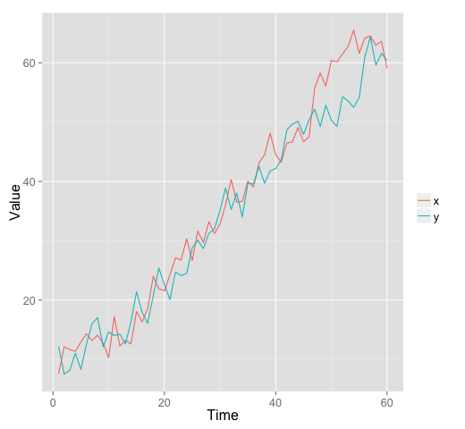
データの生成。xとyは同じようなシステムプロセスをもつが、データは別々になっている。

set.seed(1234)

N.t <- 60
mu.x <- numeric(N.t)
x <- numeric(N.t)
mu.y <- numeric(N.t)
y <- numeric(N.t)
s1 <- 2
s2 <- 1

mu.x[1] <- mu.y[1] <- 10

for (t in 1:(N.t - 1)) {
  x[t] <- rnorm(1, mu.x[t], s1)
  mu.x[t + 1] <- rnorm(1, mu.x[t] + 1, s2)
  y[t] <- rnorm(1, mu.y[t], s1)
  mu.y[t + 1] <- rnorm(1, mu.y[t] + 1, s2)
}
x[N.t] <- rnorm(1, mu.x[N.t - 1], s1)
y[N.t] <- rnorm(1, mu.y[N.t - 1], s1)

グラフを表示。

## Plot
library(ggplot2)

df1 <- data.frame(time = 1:N.t, x = x, y = y)

p1 <- ggplot(df1)
p1 + geom_line(aes(x = rep(time, 2), y = c(x, y),
                   color = rep(c("x", "y"), each = N.t))) +
  xlab("Time") + ylab("Value") +
  guides(color = guide_legend(title = "")) +
  theme_gray(base_size = 16)

p1 + geom_point(aes(x = x, y = y)) +
  theme_gray(base_size = 16)

このようになる。

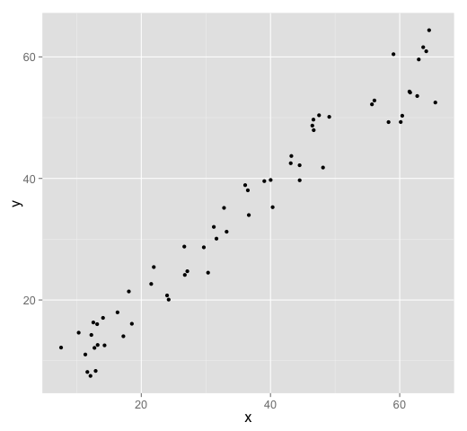
相関係数はこのとおり。

> cor.test(x, y)
	Pearson's product-moment correlation

data:  x and y
t = 35.4874, df = 58, p-value < 2.2e-16
alternative hypothesis: true correlation is not equal to 0
95 percent confidence interval:
 0.9628664 0.9866945
sample estimates:
      cor 
0.9777384 

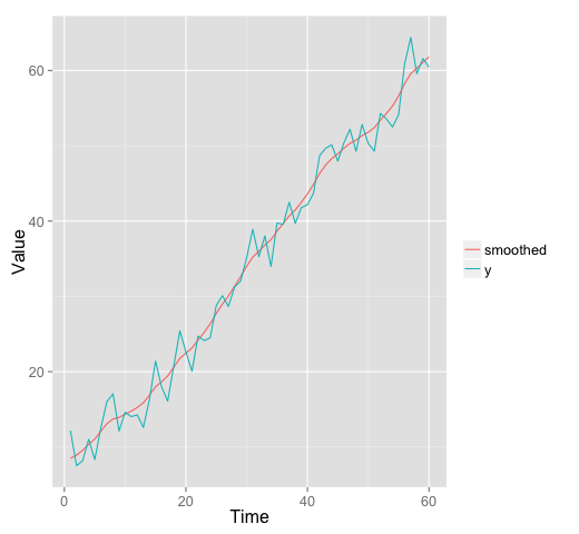
yを、xを含めないローカル線形トレンドモデルにあてはめ。

## Local linear trend model
model1 <- SSModel(y ~ SSMtrend(degree = 2,
                               Q = list(matrix(NA), matrix(NA))),
                  data = df1, H = matrix(NA))
fit1 <- fitSSM(model1, inits = c(1, 1, 1))
out1 <- KFS(fit1$model, smoothing = c("state", "mean"))
df1$smooth <- fitted(out1)

グラフ表示。

p1 <- ggplot(df1)
p1 + geom_line(aes(x = rep(time, 2), y = c(y, smooth),
                   color = rep(c("y", "smoothed"), each = N.t))) +
  xlab("Time") + ylab("Value") +
  guides(color = guide_legend(title = "")) +
  theme_gray(base_size = 16)

さらにxとの回帰を組み込んだモデル。

model2 <- SSModel(y ~ x + SSMtrend(degree = 2,
                                   Q = list(matrix(NA), matrix(NA))),
                  data = df1, H = matrix(NA))
fit2 <- fitSSM(model2, inits = c(1, 1, 1, 1))
out2 <- KFS(fit2$model, smoothing = c("state", "mean"))

結果表示。n = 60の状態だが、xの係数はすべておなじはず。係数の推定値は0.04613で、標準誤差0.12858より あきらかにちいさい。

> print(out2)

 Smoothed values of states and standard errors at time n = 60:
       Estimate  Std. Error
x       0.04613   0.12858  
level  58.85695   8.32678  
slope   0.85971   0.16395  

尤度を比較する。

> print(out1$logLik)
[1] -142.331
> print(out2$logLik)
[1] -143.4047

xとの回帰を組み込んだモデルの方が尤度が小さい。ということで、単純に相関係数を計算すると有意な相関があるが、状態空間モデルで解析してみると、xの効果はyにはあるとはいえないことがわかる。

タグ：R KFAS