Stan: 欠測値の推定 [統計]
Stanのマニュアルを見ながら、欠測値の推定をやってみたのでメモ。
下のようなデータがあったとする。
 [1,] -3.0150087  0.8224304  -3.5474533
 [2,] -2.0796367  1.0398335  -1.4325317
 [3,] -2.2329870  1.1210478  -0.9401105
 [4,] -2.8172679 -1.5561365 -10.7433671
 [5,] -1.2279092  0.5832502  -0.6014049
 [6,] -2.1656119  1.5512307   0.3979848
 [7,] -1.0271256  1.2240323   1.4461063
 [8,] -0.2834660  1.1681719   3.3905226
 [9,] -1.7447630  2.0518301   3.1254418
[10,] -1.6334189  1.3834487   0.6055146
[11,] -0.8192108  2.2543968   5.4048861
[12,] -1.3568079  1.6684795   1.3956139
[13,] -0.7046781  1.7936807   3.1889774
[14,] -1.8120819  3.2153371   4.3616880
[15,] -0.4087949  3.8920564  10.9359402
[16,] -2.0551791  2.0741935   1.9299091
[17,] -1.1615289  3.7516962   7.7151888
[18,] -1.8406299  1.7685126   1.7925101
[19,] -1.3740456  2.5434525   4.5620398
[20,] -1.3664153  1.0109986   1.2107255
[21,] -1.3189724  2.3155315   3.3852880
[22,] -2.6820334  4.4423275   8.2837741
[23,] -2.7232567  2.5496929   2.7953275
[24,] -0.3264740  1.9707566   5.1704778
[25,] -2.5957556  1.1692166  -2.3269244
[26,] -0.8401562  3.2464344   8.2907162
[27,] -1.8825776  0.6242447  -1.4520879
[28,] -1.7407786  1.6688916   1.5948284
[29,] -1.6176379  2.9809115   5.5199313
[30,] -2.7114817  4.1907706   7.1706177
これが、下のようにいくつかが欠測になったとする。
              x1         x2           y
 [1,] -3.0150087  0.8224304  -3.5474533
 [2,]         NA  1.0398335  -1.4325317
 [3,] -2.2329870  1.1210478  -0.9401105
 [4,] -2.8172679 -1.5561365 -10.7433671
 [5,] -1.2279092  0.5832502  -0.6014049
 [6,] -2.1656119  1.5512307   0.3979848
 [7,] -1.0271256  1.2240323   1.4461063
 [8,] -0.2834660  1.1681719   3.3905226
 [9,] -1.7447630  2.0518301   3.1254418
[10,]         NA         NA   0.6055146
[11,] -0.8192108  2.2543968   5.4048861
[12,] -1.3568079  1.6684795   1.3956139
[13,]         NA  1.7936807   3.1889774
[14,]         NA  3.2153371   4.3616880
[15,] -0.4087949         NA  10.9359402
[16,] -2.0551791  2.0741935   1.9299091
[17,] -1.1615289  3.7516962   7.7151888
[18,] -1.8406299  1.7685126   1.7925101
[19,]         NA  2.5434525   4.5620398
[20,] -1.3664153         NA   1.2107255
[21,] -1.3189724         NA   3.3852880
[22,] -2.6820334  4.4423275   8.2837741
[23,]         NA  2.5496929   2.7953275
[24,] -0.3264740         NA   5.1704778
[25,] -2.5957556  1.1692166  -2.3269244
[26,]         NA  3.2464344   8.2907162
[27,] -1.8825776  0.6242447  -1.4520879
[28,] -1.7407786  1.6688916   1.5948284
[29,] -1.6176379  2.9809115   5.5199313
[30,] -2.7114817  4.1907706   7.1706177
このようなデータで、欠測部分をStanで推定してみる。Reference Manual の 7.1節に例題があるが、Stanでは欠測値を扱えないので、欠測値の部分をパラメーターにして計算する。RとStanのコードは以下のとおり。x1_missとx2_missの事前分布を指定しないと収束しない。
# Data
set.seed(17)
N <- 30
x1 <- rnorm(N, -2, 1)
x2 <- rnorm(N, 2, 1)
y <- 2 * x1 + 3 * x2 + rnorm(N, 0, 0.5)

# save original values
ox1 <- x1
ox2 <- x2
oy <- y

# Missing data
x1[sample(N, 7)] <- NA
x2[sample(N, 5)] <- NA

print(cbind(x1, x2, y))

## sort
idx0 <- (1:N)[!is.na(x1) & !is.na(x2)]
idx1 <- (1:N)[!is.na(x1) & is.na(x2)]
idx2 <- (1:N)[is.na(x1) & !is.na(x2)]
idx3 <- (1:N)[is.na(x1) & is.na(x2)]

x1 <- x1[c(idx0, idx1, idx2, idx3)]
x2 <- x2[c(idx0, idx1, idx2, idx3)]
y <- y[c(idx0, idx1, idx2, idx3)]
ox1 <- ox1[c(idx0, idx1, idx2, idx3)]
ox2 <- ox2[c(idx0, idx1, idx2, idx3)]
oy <- oy[c(idx0, idx1, idx2, idx3)]

print(cbind(x1, x2, y))

## Stan
library(rstan)
library(parallel)

stancode <- "
data {
  int<lower=0> N;
  int<lower=0> M0;
  int<lower=0> M1;
  int<lower=0> M2;
  real x1[M0 + M1];
  real x2[M0 + M2];
  real y[N];
}
transformed data {
  int M3;
  M3 <- N - M0 - M1 - M2;
}
parameters {
  real x1_miss[M2 + M3];
  real x2_miss[M1 + M3];
  real beta[3];
  real<lower=0> sigma;
}
model {
  for (i in 1:M0) {
    y[i] ~ normal(beta[1] +
                    beta[2] * x1[i] +
                    beta[3] * x2[i],
                  sigma);
  }
  for (i in (M0 + 1):(M0 + M1)) {
    y[i] ~ normal(beta[1] +
                    beta[2] * x1[i] +
                    beta[3] * x2_miss[i - M0],
                  sigma);
  }
  for (i in (M0 + 1):(M0 + M2)) {
    y[M1 + i] ~ normal(beta[1] +
                         beta[2] * x1_miss[i - M0] +
                         beta[3] * x2[i],
                       sigma);
  }
  for (i in 1:M3) {
    y[M0 + M1 + M2 + i] ~ normal(beta[1] +
                                   beta[2] * x1_miss[M2 + i] +
                                   beta[3] * x2_miss[M1 + i],
                                 sigma);
  }
  x1_miss ~ normal(mean(x1), sd(x1));
  x2_miss ~ normal(mean(x2), sd(x2));
}
"

model <- stan_model(model_code = stancode)

data <- list(N = N,
             M0 = length(idx0),
             M1 = length(idx1),
             M2 = length(idx2),
             x1 = x1[!is.na(x1)],
             x2 = x2[!is.na(x2)],
             y = y)
seeds <- c(1, 2, 3, 5)

sflist <- mclapply(1:4,
                    function(i) {
                        sampling(model,
                                 data = data, seed = seeds[i],
                                 chains = 1, iter = 2000)},
                   mc.cores = 4)
fit <- sflist2stanfit(sflist)

##
library(ggplot2)

samp <- extract(fit, pars = c("x1_miss", "x2_miss"))
q.x1_miss <- apply(samp$x1_miss, 2, quantile, probs = c(0.025, 0.5, 0.975))
q.x2_miss <- apply(samp$x2_miss, 2, quantile, probs = c(0.025, 0.5, 0.975))

df <- data.frame(var = c(rep("x1_miss", ncol(q.x1_miss)),
                         rep("x2_miss", ncol(q.x2_miss))),
                 x = as.factor(c(1:ncol(q.x1_miss),
                                 1:ncol(q.x2_miss))),
                 orig = c(ox1[is.na(x1)], ox2[is.na(x2)]),
                 low = c(q.x1_miss[1, ], q.x2_miss[1, ]),
                 med = c(q.x1_miss[2, ], q.x2_miss[2, ]),
                 high = c(q.x1_miss[3, ], q.x2_miss[3, ]))
p <- ggplot(df) +
    geom_pointrange(aes(x = x, y = med, ymax = high, ymin = low),
                    colour = "red", size = 1, alpha = 0.8) +
    geom_point(aes(x = x, y = orig), shape = 3, size = 4,
               colour = "black", alpha = 1) +
    xlab("x") + ylab("value") +
    facet_wrap(~ var, scales = "free_x")
print(p)
結果
Inference for Stan model: stancode.
4 chains, each with iter=2000; warmup=1000; thin=1;
post-warmup draws per chain=1000, total post-warmup draws=4000.

            mean se_mean   sd  2.5%   25%   50%   75% 97.5% n_eff Rhat
x1_miss[1] -2.19    0.00 0.27 -2.71 -2.37 -2.19 -2.01 -1.65  4000    1
x1_miss[2] -1.12    0.00 0.26 -1.62 -1.29 -1.12 -0.96 -0.62  2912    1
x1_miss[3] -2.50    0.00 0.27 -3.03 -2.67 -2.50 -2.34 -1.97  4000    1
x1_miss[4] -1.52    0.00 0.26 -2.03 -1.68 -1.52 -1.36 -1.00  4000    1
x1_miss[5] -2.33    0.00 0.26 -2.84 -2.50 -2.32 -2.15 -1.81  4000    1
x1_miss[6] -0.79    0.00 0.28 -1.35 -0.96 -0.78 -0.61 -0.24  3839    1
x1_miss[7] -1.80    0.02 0.76 -3.32 -2.30 -1.81 -1.30 -0.32  2520    1
x2_miss[1]  3.91    0.00 0.21  3.51  3.78  3.91  4.05  4.33  3482    1
x2_miss[2]  1.34    0.00 0.18  0.97  1.22  1.34  1.46  1.68  4000    1
x2_miss[3]  2.03    0.00 0.18  1.67  1.91  2.02  2.14  2.40  4000    1
x2_miss[4]  1.95    0.00 0.20  1.56  1.83  1.95  2.08  2.34  3049    1
x2_miss[5]  1.43    0.01 0.53  0.38  1.08  1.44  1.78  2.47  2391    1
beta[1]     0.00    0.01 0.36 -0.72 -0.23 -0.01  0.23  0.70  1946    1
beta[2]     2.01    0.00 0.16  1.70  1.91  2.02  2.11  2.34  2209    1
beta[3]     2.98    0.00 0.09  2.81  2.92  2.98  3.04  3.15  3013    1
sigma       0.52    0.00 0.10  0.37  0.45  0.51  0.58  0.76  1383    1
lp__        0.65    0.14 3.86 -8.15 -1.71  1.03  3.49  6.76   795    1

Samples were drawn using NUTS(diag_e) at Sat Mar  7 14:59:25 2015.
For each parameter, n_eff is a crude measure of effective sample size,
and Rhat is the potential scale reduction factor on split chains (at
convergence, Rhat=1).
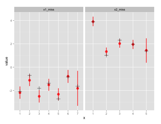
赤の点と線が事後分布の中央値および95%信用区間、黒の十字が元のデータ。
だいたいうまく推定できているが、x1とx2の両方が欠測になったx1_miss[7]とx2_miss[5]では信用区間が広くなっている。
タグ:RStan


コメント 0