2次元でのStanによるCARモデルのテスト [統計]
berobero11さんのStanによるCARモデルを2次元でためしてみたテストです。
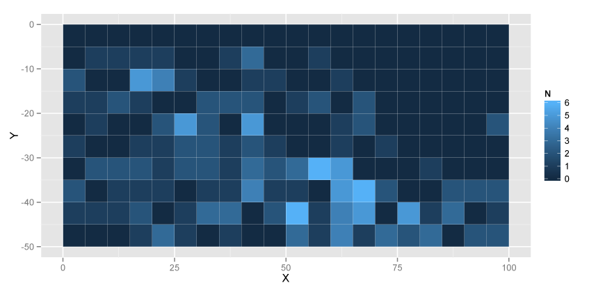
使用したデータは、銀閣寺山国有林(京都市左京区)で取得したアラカシという木の分布データです。50m×100mの調査地を5m×5mのメッシュに分割して、それぞれのメッシュに含まれるアラカシの個体数(株数)を測定しました。方法の詳細は、伊東(2007)をご覧ください。1993年のデータを使用しました。
データ→Qglauca.csv
図示してみると以下のようになります。
## http://cse.ffpri.affrc.go.jp/hiroki/stat/Qglauca.csv
qg <- read.csv("Qglauca.csv")

## Plot
library(ggplot2)
ggplot(qg) +
    geom_tile(aes(x = X + 2.5, y = Y - 2.5, fill = N)) +
    xlab("X") + ylab("Y")
まずはOpenBUGSでCARモデルにあてはめをしてみます。
## Conditional Autoregression Model
## adjacent plots
adj <- c(2, 11,         # 1
         c(sapply(2:9, function(i) i + c(-1, 1, 10))),           # 2--9
         9, 20,         # 10

         c(sapply(seq(0, 170, 10),
                  function(j) j + c(1, 12, 21,
                                    c(sapply(2:9,
                                             function(i) i + c(0, 9, 11, 20))),
                                    10, 19, 30))), # 10--190

         181, 192,      # 191
         c(sapply(2:9, function(i) i + c(180, 189, 191))),     # 192--199
         190, 199)    # 200
num.adj <- c(2, rep(3, 8), 2,
             rep(c(3, rep(4, 8), 3), 18),
             2, rep(3, 8), 2)
weights <- rep(1, length(adj))

## OpenBUGS
library(R2OpenBUGS)
## OS X (Darwin) なら/Applications/Wine.appを使用
## Linuxなら/usr/local/bin/OpenBUGSを使用
uname <- system("uname", intern = TRUE)
if (uname == "Darwin") {
  Sys.setenv(DYLD_FALLBACK_LIBRARY_PATH="/usr/x11/lib")
  kOpenBUGS <- paste(Sys.getenv("HOME"),
                     ".wine/drive_c/Program\ Files",
                     "OpenBUGS/OpenBUGS322/OpenBUGS.exe", sep = "/")
  kWine <- "/Applications/Wine.app/Contents/Resources/bin/wine"
  kWinePath <- "/Applications/Wine.app/Contents/Resources/bin/winepath"
  useWine <- TRUE
  debug <- TRUE
} else if (uname == "Linux") {
  kOpenBUGS <- "/usr/local/bin/OpenBUGS"
  kWine <- NULL
  kWinePath <- NULL
  useWine <- FALSE
  debug <- FALSE
}

## BUGS model
bugs.model <- "
var
  ## data
  N_site,               # number of subquadrats
  Y[N_site],            # stem number of Q.glauca
  AdjNum[N_site],       # number of adjacent plots
  N_Adj,                # length of Adj[]
  Adj[N_Adj],           # adjacent plots
  Weights[N_Adj],       # weights
  ## parameters
  beta,                 # intercept
  lamdba[N_site],       # mean number of individuals
  r[N_site]             # spatial error
  tau,
  sigma;
model {
  for (i in 1:N_site) {
    Y[i] ~ dpois(lambda[i]);
    log(lambda[i]) <- beta + r[i];
  }
  r[1:N_site] ~ car.normal(Adj[], Weights[], AdjNum[], tau);
  beta ~ dnorm(0, 1.0E-4);
  tau <- 1 / (sigma * sigma);
  sigma ~ dunif(0, 1.0E+4);
}"
model.file <- "Qglauca_bugs.txt"
cat(bugs.model, file = model.file)

## parameters to save
params <- c("beta", "sigma", "lambda")
iter <- 7000
burnin <- 2000
thin <- 5

##
data <- list(N_site = nrow(qg),
             Y = qg$N,
             AdjNum = num.adj,
             N_Adj = length(num.adj),
             Adj = adj,
             Weights = weights)
inits <- list(list(beta = 0, sigma = 1),
              list(beta = 1, sigma = 2),
              list(beta = 3, sigma = 0.1))
samp <- bugs(data = data,
             model.file = model.file,
             inits = inits,
             parameters = params,
             n.chains = 3,
             n.iter = iter, n.burnin = burnin, n.thin = thin,
             OpenBUGS = kOpenBUGS,
             useWINE = useWine,
             WINE = kWine,
             WINEPATH = kWinePath,
             debug = debug)
結果
> print(samp, digits = 3)
Inference for Bugs model at "Qglauca_bugs.txt",
Current: 3 chains, each with 7000 iterations (first 2000 discarded), n.thin = 5
Cumulative: n.sims = 15000 iterations saved
               mean     sd    2.5%     25%     50%     75%   97.5%  Rhat n.eff
beta         -0.528  0.130  -0.800  -0.612  -0.522  -0.438  -0.285 1.001  5500
sigma         1.168  0.175   0.848   1.048   1.158   1.280   1.537 1.001 15000
[...]
deviance    434.622 15.764 404.300 424.000 434.300 444.900 466.600 1.001  6400

For each parameter, n.eff is a crude measure of effective sample size,
and Rhat is the potential scale reduction factor (at convergence, Rhat=1).

DIC info (using the rule, pD = Dbar-Dhat)
pD = 2.4 and DIC = 437.0
DIC is an estimate of expected predictive error (lower deviance is better).
library(ggplot2)

N_site <- nrow(qg)
N = qg$N
ggplot(data.frame(x = 1:N_site,
                  y = N,
                  ymean = samp$mean$lambda,
                  ymax = apply(samp$sims.list$lambda, 2, quantile, 0.975),
                  ymin = apply(samp$sims.list$lambda, 2, quantile, 0.025))) +
    geom_point(aes(x = x, y = y)) +
    geom_pointrange(aes(x = x, y = ymean, ymax = ymax, ymin = ymin),
                    colour = "red", alpha = 0.5, shape = 3) +
    xlab("Index") + ylab("N") + ylim(0, 9)
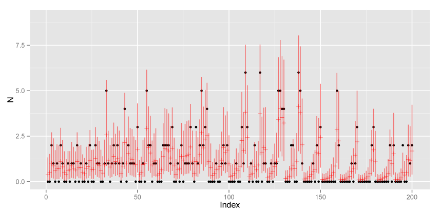
黒が実測値、赤が事後分布の平均値と95%信用区間です。
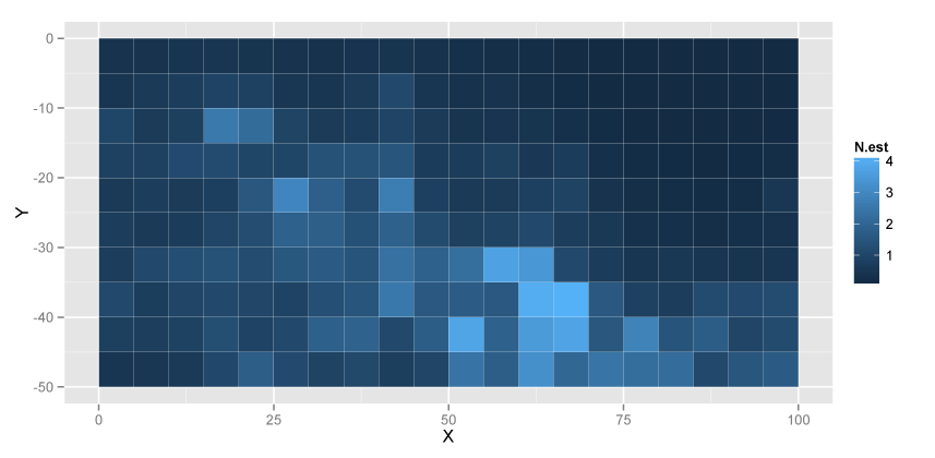
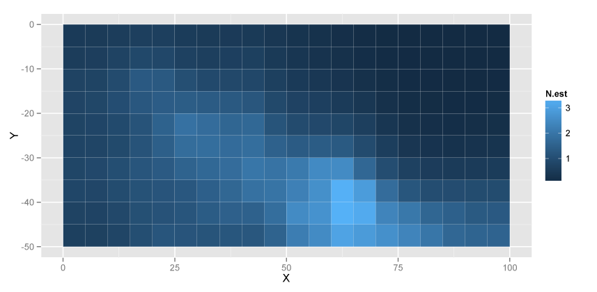
ggplot(data.frame(x = qg$X, y = qg$Y,
                  N.est = samp$mean$lambda)) +
    geom_tile(aes(x = x + 2.5, y = y - 2.5, fill = N.est)) +
    xlab("X") + ylab("Y")
つづいて、Stanで。Stanのコードはほぼberobero11さんのコードそのままです。CAR.stanというファイル名で保存。
/*
  CAR.stan
  CAR model created by @berobero11
  http://heartruptcy.blog.fc2.com/blog-entry-141.html
*/
data {
   int<-lower=1> N_site;
   int<-lower=1> N_Adj;
   int<-lower=0> Y[N_site];
   int<-lower=1> Adj[N_Adj];
   real<-lower=0> Weight[N_Adj];
   int<-lower=1> Offset[N_site, 2];
}

parameters {
   real r0[N_site-1];
   real beta;
   real<-lower=0> sigma;
}

transformed parameters {
   real r[N_site];
   real s[N_site];
   real mu[N_site];

   for (j in 1:(N_site-1))
      r[j] <- r0[j];
   r[N_site] <- -sum(r0);

   for (j in 1:N_site) {
      real sum_x;
      real sum_w;
      sum_x <- 0.0;
      sum_w <- 0.0;
      for (i in Offset[j, 1]:Offset[j, 2]) {
         sum_x <- sum_x + Weight[i] * r[Adj[i]];
         sum_w <- sum_w + Weight[i];
      }
      mu[j] <- sum_x / sum_w;
      s[j] <- sigma / sqrt(sum_w);
   }
}

model {
   for (j in 1:N_site) {
     Y[j] ~ poisson_log(beta + r[j]);
     r[j] ~ normal(mu[j], s[j]);
   }
   beta ~ normal(0, 1.0e+2);
   sigma ~ uniform(0, 1.0e+4);
}

generated quantities {
   real<-lower=0> Y_mean[N_site];
   for (j in 1:N_site)
      Y_mean[j] <- exp(beta + r[j]);
}
OS X MavericksでR 3.1.0だと、RStanがこけるので、CmdStanを使用しました。
## データを用意
qg <- read.csv("Qglauca.csv")

adj <- c(2, 11,         # 1
         c(sapply(2:9, function(i) i + c(-1, 1, 10))),           # 2--9
         9, 20,         # 10

         c(sapply(seq(0, 170, 10),
                  function(j) j + c(1, 12, 21,
                                    c(sapply(2:9,
                                             function(i) i + c(0, 9, 11, 20))),
                                    10, 19, 30))), # 10--190

         181, 192,      # 191
         c(sapply(2:9, function(i) i + c(180, 189, 191))),     # 192--199
         190, 199)    # 200
num.adj <- c(2, rep(3, 8), 2,
             rep(c(3, rep(4, 8), 3), 18),
             2, rep(3, 8), 2)
weights <- rep(1, length(adj))
N_site <- nrow(qg)
offset2 <- offset1 <- rep(NA, N_site)
offset1[1] <- 1
for (i in 2:N_site) {
  offset1[i] <- 1 + sum(num.adj[1:(i - 1)])
}
for (i in 1:(N_site - 1)) {
  offset2[i] <- offset1[i + 1] - 1
}
offset2[N_site] <- length(adj)
Offset <- cbind(offset1, offset2)
colnames(Offset) <- NULL

Y <- qg$N
Adj <- adj
N_Adj <- length(Adj)
Weight <- weights

dump(c("Y", "N_site", "N_Adj", "Adj", "Weight", "Offset"),
     file = "Qglauca_dump.R")
CAR.stanをコンパイルしておいて、以下のシェルスクリプトを実行。
#!/bin/sh
ITER=5000
WARMUP=2000
THIN=5
DATA=Qglauca_dump.R
OUT=Qglauca

./CAR sample num_samples=${ITER} num_warmup=${WARMUP} thin=${THIN} \
	id=1 data file=${DATA} random seed=123 output file=${OUT}_1.csv \
	refresh=1000 &
./CAR sample num_samples=${ITER} num_warmup=${WARMUP} thin=${THIN} \
	id=2 data file=${DATA} random seed=345 output file=${OUT}_2.csv \
	refresh=1000 &
./CAR sample num_samples=${ITER} num_warmup=${WARMUP} thin=${THIN} \
	id=3 data file=${DATA} random seed=567 output file=${OUT}_3.csv \
	refresh=1000 &
結果のとりこみ
library(coda)

fit <- list()
for (i in 1:3) {
  fit[[i]] <- as.mcmc(read.csv(paste("Qglauca_", i, ".csv", sep = ""),
                               comment = "#"))
}
fit.mcmc.list <- as.mcmc.list(fit)

summary(fit.mcmc.list[, c("beta", "sigma")])
gelman.diag(fit.mcmc.list[, c("beta", "sigma")],
            multivariate = FALSE)
params <- colnames(fit[[1]])
pos.Y_mean <- match("Y_mean.1", params)
Y_mean <- fit.mcmc.list[, pos.Y_mean:(pos.Y_mean + N_site - 1)]
summary.Y_mean <- summary(Y_mean)
結果の表示
> summary(fit.mcmc.list[, c("beta", "sigma")])

Iterations = 1:1000
Thinning interval = 1
Number of chains = 3
Sample size per chain = 1000

1. Empirical mean and standard deviation for each variable,
   plus standard error of the mean:

         Mean     SD Naive SE Time-series SE
beta  -0.4753 0.1344 0.002454       0.005060
sigma  0.3728 0.1036 0.001891       0.006123

2. Quantiles for each variable:

         2.5%     25%     50%     75%   97.5%
beta  -0.7532 -0.5609 -0.4685 -0.3853 -0.2306
sigma  0.2145  0.3006  0.3571  0.4264  0.6237

> gelman.diag(fit.mcmc.list[, c("beta", "sigma")],
+             multivariate = FALSE)
Potential scale reduction factors:

      Point est. Upper C.I.
beta           1       1.01
sigma          1       1.02
グラフを表示
library(ggplot2)
ggplot(data.frame(x = 1:N_site,
                  y = Y,
                  ymean = summary.Y_mean$statistic[, "Mean"],
                  ymax = summary.Y_mean$quantiles[, "97.5%"],
                  ymin = summary.Y_mean$quantiles[, "2.5%"])) +
    geom_point(aes(x = x, y = y)) +
    geom_pointrange(aes(x = x, y = ymean, ymax = ymax, ymin = ymin),
                  colour = "red", alpha = 0.5, shape = 3) +
    xlab("Index") + ylab("N") + ylim(0, 9)
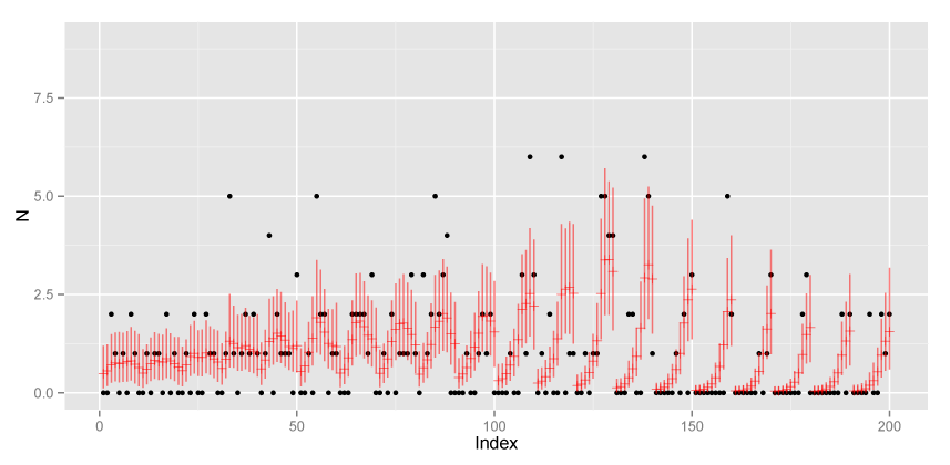
黒が実測値、赤が事後分布の平均値と95%信用区間です。
ggplot(data.frame(x = qg$X, y = qg$Y,
                  N.est = summary.Y_mean$statistic[, "Mean"])) +
    geom_tile(aes(x = x + 2.5, y = y - 2.5, fill = N.est)) +
    xlab("X") + ylab("Y")
どうもStanの方が空間誤差の分散が小さく推定されるようです。 と、ここまで来たところで まだ原因は追及していません。どこか間違えているかも。


コメント 0