GLMM説明用データ

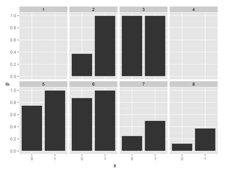
GLMMを説明するデータをつくってみた。まずは二項分布。

library(ggplot2)
library(glmmML)

inv.logit <- function(x) {
	1 / (1 + exp(-x))
}

set.seed(1234)

n.block <- 8
n.measure <- 16

block <- rep(1:n.block, each = n.measure)
x <- rep(rep(c(0, 1), each = n.measure / 2), n.block)
err.bl <- rep(rnorm(n.block, 0, 3.0), each = n.measure)
y.m <- inv.logit(-1 + 2 * x + err.bl)
y <- rbinom(length(y.m), 1, y.m)
data <- data.frame(block = block, x = x, y = y)
tdata <- melt(tapply(data$y, list(data$block, data$x), mean))

ggplot(tdata, aes(y = value, x = as.factor(X2)), facet = X1) +
	geom_bar() + facet_wrap(~ X1, nrow = 2) +
	xlab("x") + ylab("p")

何もかんがえずに割合で分散分析

> summary(aov(value ~ X2, data = tdata))
            Df  Sum Sq Mean Sq F value Pr(>F)
X2           1 0.14062 0.14062  0.7742 0.3938
Residuals   14 2.54297 0.18164               

ブロックを考慮せずGLMを適用

> summary(glm(y ~ x,  family = binomial, data = data))

Call:
glm(formula = y ~ x, family = binomial, data = data)

Deviance Residuals: 
    Min       1Q   Median       3Q      Max  
-1.3711  -1.0469   0.9953   0.9953   1.3138  

Coefficients:
            Estimate Std. Error z value Pr(>|z|)  
(Intercept)  -0.3151     0.2531  -1.245   0.2132  
x             0.7598     0.3601   2.110   0.0349 *
---
Signif. codes:  0 ‘***’ 0.001 ‘**’ 0.01 ‘*’ 0.05 ‘.’ 0.1 ‘ ’ 1 

(Dispersion parameter for binomial family taken to be 1)

    Null deviance: 177.32  on 127  degrees of freedom
Residual deviance: 172.79  on 126  degrees of freedom
AIC: 176.79

Number of Fisher Scoring iterations: 4

GLMMを適用

> glmmML(y ~ x, cluster = block, family = binomial, data = data)

Call:  glmmML(formula = y ~ x, family = binomial, data = data, cluster = block) 


              coef se(coef)       z Pr(>|z|)
(Intercept) -1.135   1.4873 -0.7632  0.44500
x            2.022   0.6654  3.0395  0.00237

Scale parameter in mixing distribution:  3.791 gaussian 
Std. Error:                              0.7296 

        LR p-value for H_0: sigma = 0:  8.646e-19 

Residual deviance: 95.81 on 125 degrees of freedom 	AIC: 101.8 

タグ：R glmm