混合効果モデル説明用データ [統計]
混合効果モデルを説明するデータをつくってみた。
コード
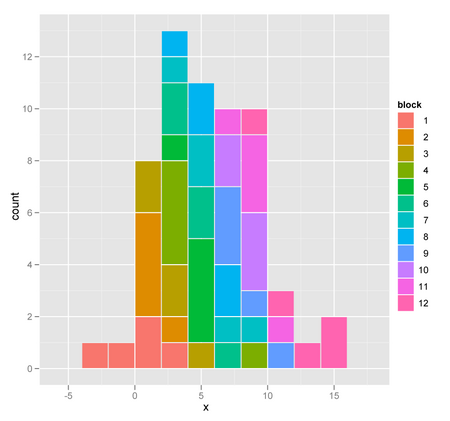
変数xのヒストグラム
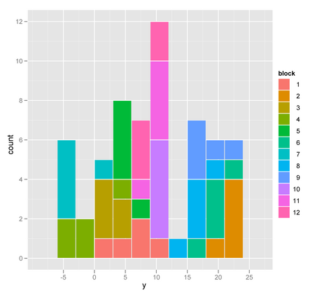
変数yのヒストグラム
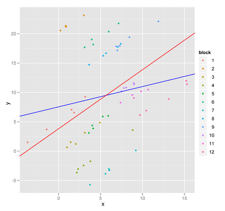
lm()とlme()の結果の比較
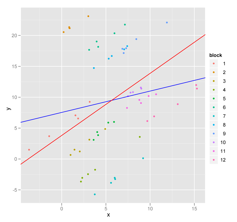
散布図と回帰直線
コード
library(nlme)
library(ggplot2)

set.seed(1234)

n.block <- 12
n.measure <- 5

block <- rep(1:n.block, each = n.measure)
x.m <- block
x <- x.m + rnorm(n.block * n.measure, 0, 2.0)
err.bl <- rep(rnorm(n.block, 0, 8.0), each = n.measure)
err <- rnorm(n.block * n.measure, 0, 0.4)
y <- 1.0 * x + err.bl + err

data <- data.frame(block = as.factor(block), x = x, y = y)

# histogram
ggplot(data) + geom_histogram(aes(x = x, fill = block), binwidth = 2)
ggplot(data) + geom_histogram(aes(x = y, fill = block), binwidth = 3)

# scatter plot
p1 <- ggplot(data, aes(x = x, y = y, colour = block)) +
      geom_point()
#print(p1)


lm1 <- lm(y ~ x, data = data)
summary(lm1)

lme1 <- lme(y ~ x, random = ~1|block, data = data, method = "ML")
summary(lme1)

# add lines
p2 <- p1 +
    geom_abline(aes(intercept = coef(lm1)[1],
                    slope = coef(lm1)[2]), colour = 4) +
    geom_abline(aes(intercept = fixef(lme1)[1],
                    slope = fixef(lme1)[2]), colour = 2)
print(p2)
変数xのヒストグラム

変数yのヒストグラム

lm()とlme()の結果の比較
>  summary(lm1)

Call:
lm(formula = y ~ x, data = data)

Residuals:
    Min      1Q  Median      3Q     Max
-14.557  -5.199  -1.008   7.797  14.535

Coefficients:
            Estimate Std. Error t value Pr(>|t|)
(Intercept)   7.5380     1.8846   4.000 0.000182 ***
x             0.3457     0.2767   1.249 0.216578
---
Signif. codes:  0 ‘***’ 0.001 ‘**’ 0.01 ‘*’ 0.05 ‘.’ 0.1 ‘ ’ 1

Residual standard error: 8.146 on 58 degrees of freedom
Multiple R-squared: 0.0262,	Adjusted R-squared: 0.009414
F-statistic: 1.561 on 1 and 58 DF,  p-value: 0.2166

>  summary(lme1)
Linear mixed-effects model fit by maximum likelihood
 Data: data
       AIC      BIC    logLik
  147.0324 155.4098 -69.51622

Random effects:
 Formula: ~1 | block
        (Intercept)  Residual
StdDev:    8.385314 0.3470586

Fixed effects: y ~ x
               Value Std.Error DF  t-value p-value
(Intercept) 3.807343 2.4672256 47  1.54317  0.1295
x           1.005746 0.0271906 47 36.98874  0.0000
 Correlation:
  (Intr)
x -0.062

Standardized Within-Group Residuals:
        Min          Q1         Med          Q3         Max
-1.81346566 -0.58107091  0.06529203  0.54893908  2.15375512

Number of Observations: 60
Number of Groups: 12
散布図と回帰直線


コメント 0