累積ロジットモデルのベイズ推定(2) [統計]
前回のつづき。今度はランダム効果の入ったデータを推定してみる。
まずはデータを用意。
# inverse logit
invlogit <- function(x) exp(x)/(1+exp(x))

set.seed(12345)
n.rank <- 5
plot <- 1:20
n.plot <- length(plot)
time <- 1:5
n.time <- length(time)
n <- n.plot * n.time
data <- expand.grid(plot = plot, time = time)
slope <- rgamma(n.plot, shape = 15^2/5^2, rate = 15/5^2)
data$slope <- rep(slope, n.time)
ranef.plot <- rnorm(n.plot, 0, 1)
ranef.time <- rnorm(n.time, 0, 1)
logit.c1 <- 7.5 - 0.5 * slope +
            ranef.plot[data$plot] + ranef.time[data$time]
data$c1 <- rbinom(n, n.rank - 1, invlogit(logit.c1)) + 1
累積データを作成して、JAGSにかける。
cum <- matrix(NA, nrow = n.plot * n.time, ncol = n.rank - 1)
cum[,1] <- as.numeric(data$c1 >= 2)
cum[,2] <- as.numeric(data$c1 >= 3)
cum[,3] <- as.numeric(data$c1 >= 4)
cum[,4] <- as.numeric(data$c1 >= 5)

library(rjags)
model <- jags.model("cumlogit_MCMC2.bug",
                    data = list(N = n, M = n.rank - 1,
                                K = n.plot, L = n.time,
                                s = data$slope, c = cum,
                                plot = data$plot, time = data$time),
                    nchain = 3, n.adapt = 10000)
post <- coda.samples(model,
                     variable = c("b", "beta", "sigma.p", "sigma.t"),
                     n.iter = 20000, thin = 20)
BUGSコード
var
  N,  # number of data
  M,  # number of ranks
  K,  # number of plots
  L,  # number of mesurements
  beta,
  b[M],
  c[N, M],
  s[N],
  plot[N], e.plot[K],
  time[N], e.time[L];

model {
  for (j in 1:M) {
    for (i in 1:N) {
      c[i, j] ~ dbern(p[i, j]);
      logit(p[i, j]) <- b[j] + beta * s[i] +
                        e.plot[plot[i]] + e.time[time[i]];
    }
    b[j] ~ dnorm(0.0, 1.0E-4);
  }

  for (i in 1:K) {
    e.plot[i] ~ dnorm(0, tau.p);
  }

  for (i in 1:L) {
    e.time[i] ~ dnorm(0, tau.t);
  }

  beta ~ dnorm(0.0, 1.0E-4);
  tau.p ~ dgamma(1.0E-3, 1.0E-3);
  tau.t ~ dgamma(1.0E-3, 1.0E-3);
  sigma.p <- 1/sqrt(tau.p);
  sigma.t <- 1/sqrt(tau.t);
}
結果
> summary(post)

Iterations = 10020:30000
Thinning interval = 20
Number of chains = 3
Sample size per chain = 1000

1. Empirical mean and standard deviation for each variable,
   plus standard error of the mean:

           Mean     SD Naive SE Time-series SE
b[1]    14.4082 2.6237 0.047902       0.195126
b[2]    11.6440 2.4110 0.044018       0.180754
b[3]    10.2122 2.3343 0.042619       0.172398
b[4]     7.4226 2.1665 0.039554       0.152169
beta    -0.7306 0.1376 0.002513       0.009946
sigma.p  2.0650 0.5855 0.010690       0.019606
sigma.t  1.6044 0.8677 0.015841       0.021022

2. Quantiles for each variable:

           2.5%     25%    50%     75%   97.5%
b[1]     9.8577 12.6381 14.235 15.9341 19.9900
b[2]     7.4117 10.0158 11.449 13.0504 16.8387
b[3]     6.1724  8.5996 10.039 11.5374 15.2372
b[4]     3.5728  5.9820  7.287  8.6834 12.0245
beta    -1.0236 -0.8163 -0.720 -0.6385 -0.4859
sigma.p  1.1528  1.6539  1.988  2.3900  3.4480
sigma.t  0.6625  1.0580  1.399  1.8622  3.8623
同じデータをdrmで解析してみる。
library(drm)
fit <- drm(c1 ~ slope + cluster(plot) + Time(time),
                data = data,
                start = c(0, 1, 2, 3, -1),
                print.level = 0)
結果
> summary(fit)
Call:
drm(formula = c1 ~ slope + cluster(plot) + Time(time), data = data,
    start = c(0, 1, 2, 3, -1), print.level = 0)

Coefficients:
                 Value Std. Error   z value
(Intercept)1 -8.707243 1.09793339 -7.930575
(Intercept)2 -7.003733 0.94661067 -7.398747
(Intercept)3 -6.134059 0.88513704 -6.930067
(Intercept)4 -4.475916 0.79272635 -5.646230
slope        -0.444208 0.05900017 -7.528927

Residual deviance: 216.881 	AIC: 226.881

Convergence code 1 in 32 iterations (See help(nlm) for details)

Correlation of Coefficients:
             (Intercept)1 (Intercept)2 (Intercept)3 (Intercept)4
(Intercept)2        0.948
(Intercept)3        0.933        0.966
(Intercept)4        0.892        0.909        0.924
slope               0.957        0.957        0.953        0.921
なんだか微妙に結果が違うが、何が原因なのだろう? 推定法の違いによるものなのか、どっか間違えているのか。切片の符号が逆なのは、モデルでの符号の与え方の違いによるものなので、それは問題ない。
データに期待値の線を重ねてプロットしてみる。
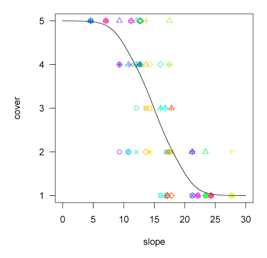
ベイズ推定によるもの
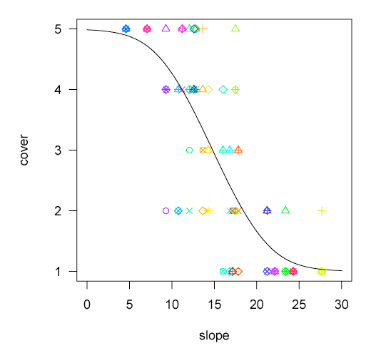
drmによるもの
タグ:累積ロジットモデル


コメント 0