glmmAK

CRANにglmmAKというパッケージが登録されていた。AKというのは作者のArnošt Komárek氏の名前からとったものか。

This package implements several generalized linear (mixed) models (GLMM) where for random effects either a conventional normal distribution is assumed or a flexible model based on penalized smoothing is used for the random effect distribution. We call the second class of models as penalized Gaussian mixture (PGM) or shortly G-spline.

通常のGLMMではrandom effectが正規分布することを仮定するが、このパッケージではpenalized Gaussian mixture (PGM)とすることができるということのようだ。で、PGMというのはG-スプラインということか。このあたり勉強不足なのでよく分からないのだが。

通常のGLMMのrandam effect項

PGMのrandom effect項

MCMCで推定をおこなうようになっている。

付属の例題(ex-Toenail)をやってみる。1) PGM GLMM, not hierarchically centered, 2) PGM GLMM, hierarchically centered, 3) Normal GLMM, not hierarchically centered, 4) Normal GLMM, hierarchically centeredの4つを比較しているが、とりあえず1)だけをやってみる。

まずはいろいろ準備。

library(glmmAK)
root <- paste(Sys.getenv("HOME"), "Documents/RData/", sep="/")
setwd(root)
data(toenail)

# 事前分布
prior.fixed <- list(mean = 0, var = 10000)

prior.gspline.Slice <- list(K = 15, delta = 0.3,
    sigma = 0.2, CARorder = 3, 
    Ldistrib = "gamma", Lequal = FALSE, Lshape = 1,
    LinvScale = 0.005, 
    AtypeUpdate = "slice") 

prior.gspline.Block <- list(K = 15, delta = 0.3,
    sigma = 0.2, CARorder = 3, 
    Ldistrib = "gamma", Lequal = FALSE, Lshape = 1,
    LinvScale = 0.005, 
    AtypeUpdate = "block") 

prior.random.gspl.nhc <- list(Ddistrib = "gamma",
    Dshape = 1, DinvScale = 0.005)

# 結果のファイルを収めるpathの準備
if (!("chToenail" %in% dir(root))) dir.create(paste(root, "chToenail", 
    sep = "")) 
dirNames <- c("PGM_nhc") 
dirPaths <- paste(root, "chToenail/", dirNames, "/", sep = "") 
for (i in 1:length(dirPaths)) { 
    if (!(dirNames[i] %in% dir(paste(root, "chToenail", sep = "")))) 
        dir.create(dirPaths[i]) 
} 
names(dirPaths) <- c("PGM_nhc") 

# 共変量
iXmat <- data.frame(trt = toenail$trt, 
    time = toenail$time, 
    trt.time = toenail$trt * toenail$time) 

# MCMCの回数
# niter × nthinが繰り返し回数となる
# 例題ではnthin = 100, nwrite = 100となっているが、それぞれ10に
nsimul <- list(niter = 4000, nthin = 10, nburn = 2000, nwrite = 10) 

MCMCを実行。

fit.PGM.nhc <- cumlogitRE(y = toenail$infect, x = iXmat, 
    cluster = toenail$idnr, intcpt.random = TRUE,
    hierar.center = FALSE, 
    C = 1, drandom = "gspline", prior.fixed = prior.fixed, 
    prior.random = prior.random.gspl.nhc,
    prior.gspline = prior.gspline.Slice, 
    nsimul = nsimul, store = list(prob = FALSE, b = TRUE), 
    dir = dirPaths["PGM_nhc"]) 

事後分布を読み込む。

chPGM.nhc <- glmmAK.files2coda(dir = dirPaths["PGM_nhc"],
    drandom = "gspline", 
    skip = 0) 

iters <- scanFH(paste(dirPaths["PGM_nhc"], "iteration.sim", sep = "")) 
betaF <- scanFH(paste(dirPaths["PGM_nhc"], "betaF.sim", sep = "")) 
betaRadj <- scanFH(paste(dirPaths["PGM_nhc"], "betaRadj.sim",
    sep = "")) 
varRadj <- scanFH(paste(dirPaths["PGM_nhc"], "varRadj.sim", sep = "")) 
chPGM.nhc <- mcmc(data.frame(Trt = betaF[, "trt"], 
    Time = betaF[, "time"], 
    Trt.Time = betaF[, "trt.time"], 
    Meanb = betaRadj[, "(Intercept)"], 
    SDb = sqrt(varRadj[, "varR.1"])), 
    start = iters[1, 1]) 
rm(list = c("iters", "betaF", "betaRadj", "varRadj")) 

結果。

summary(chPGM.nhc) 

Iterations = 2001:4000
Thinning interval = 1 
Number of chains = 1 
Sample size per chain = 2000 

1. Empirical mean and standard deviation for each variable,
   plus standard error of the mean:

            Mean      SD  Naive SE Time-series SE
Trt      -0.1707 0.55305 0.0123667       0.038592
Time     -0.3888 0.04393 0.0009823       0.001471
Trt.Time -0.1364 0.06750 0.0015093       0.002118
Meanb    -1.6728 0.42032 0.0093987       0.048364
SDb       4.0355 0.40676 0.0090954       0.032822

2. Quantiles for each variable:

            2.5%     25%     50%      75%     97.5%
Trt      -1.2368 -0.5494 -0.1756  0.20957  0.914094
Time     -0.4759 -0.4183 -0.3876 -0.35809 -0.308134
Trt.Time -0.2688 -0.1810 -0.1373 -0.08957 -0.005997
Meanb    -2.5440 -1.9513 -1.6625 -1.38506 -0.897988
SDb       3.2792  3.7500  4.0270  4.29516  4.873613

plot(chPGM.nhc) 

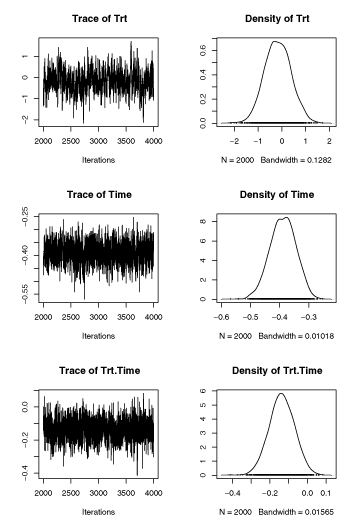
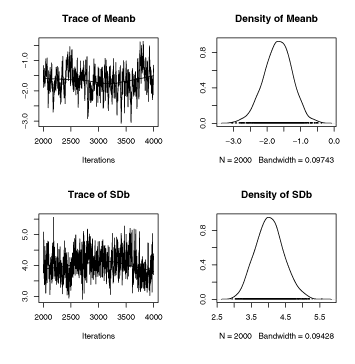
lmerと比較してみる。

library(lme4)
glmm.lmer <- lmer(infect ~ trt + time + trt:time + (1|idnr),
    family=binomial, data=toenail, method="Laplace")

Generalized linear mixed model fit using Laplace 
Formula: infect ~ trt + time + trt:time + (1 | idnr) 
   Data: toenail 
 Family: binomial(logit link)
  AIC  BIC logLik deviance
 1266 1293 -627.8     1256
Random effects:
 Groups Name        Variance Std.Dev.
 idnr   (Intercept) 20.867   4.568   
number of obs: 1908, groups: idnr, 294

Estimated scale (compare to  1 )  1.623704 

Fixed effects:
            Estimate Std. Error z value Pr(>|z|)    
(Intercept) -2.51388    0.46275  -5.432 5.56e-08 ***
trt         -0.30664    0.66293  -0.463   0.6437    
time        -0.40044    0.04520  -8.859  < 2e-16 ***
trt:time    -0.13629    0.07361  -1.851   0.0641 .  
---
Signif. codes:  0 ‘***’ 0.001 ‘**’ 0.01 ‘*’ 0.05 ‘.’ 0.1 ‘ ’ 1 

Correlation of Fixed Effects:
         (Intr) trt    time  
trt      -0.698              
time     -0.277  0.193       
trt:time  0.170 -0.278 -0.614

タグ：glmm glmmAK